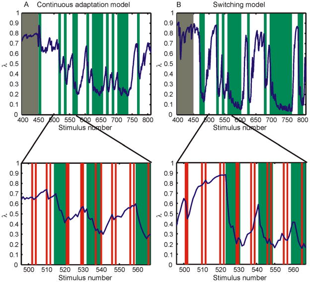
Figure 11.

Simulated learning by a Bayesian model. (A) The mean of the posterior on λ as a function of stimulus number for a simulated subject using the continuous adaptation mechanism in Experiments 4 or 5 (1 is the first stimulus of the baseline session, 451 is the first stimulus of the second session). The simulated subject was presented with stimuli in randomized order as generated by the experimental parameters for Experiments 4 and 5. White indicates epochs containing context stimuli that are circles, green represents epochs in which context stimuli were randomly shaped ellipses. Red lines indicate test stimuli containing 5° conflicts between the slant suggested by the compression cue and the slant suggested by binocular disparities. (For optical reasons, these are not shown in the upper panels, but only in the lower panels, which represent enlarged cutouts from the upper ones.) (B) The results for a simulated subject using the switching mechanism. With each stimulus presentation, the model updates a posterior probability distribution on λ, given the previous and current sensory data. The posterior probability distribution on surface slant is computed by averaging the posterior density functions for slant over this distribution of values of λ. While the model does not explicitly estimate λ – rather, it uses the posterior on λ to compute estimates of slant – the mean of the posterior serves as a good guide to tracking the dynamics of the two models.