Figure 1.

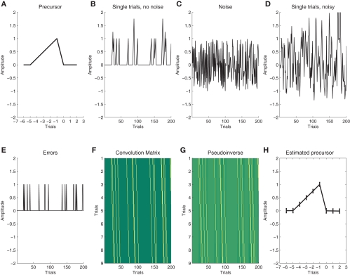
Illustration of deconvolution of latent sequential effects. (A) We assume a latent precursor signal that gradually evolves across trials and precedes each error; (B) In order to illustrate a noiseless sequence of single trials we convolve a vector with 10% errors at random instances, note the summation of overlapping sequences; (C) for real data, we assume additional noise; (D) Convolution of the noisy data (C+E) with (A) yields the simulated single-trial data that are used for deconvolution; (E) In order to deconvolve the data, we use a “Stick”-function that describes the occurrence of errors; (F) stacking the stick function at different lags is the convolution matrix; (G) we then take the pseudo-inverse of (F) and multiply the resulting matrix with the noisy data (D); (H) The product is an estimate of the precursor. In this figure, we show the average across 100 runs, error bars indicate the ±1 standard deviation around the mean.