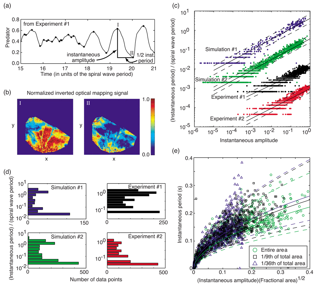
FIG. 11.

(Color online) (a) Definitions of instantaneous period and amplitude illustrated using a portion of experiment No. 1 data (see below). Asterisks mark the calculated local extrema of the data. (b) Optical mapping snapshots of the membrane potential (red = activated) in a right ventricular endocardial preparation taken at the two times marked as “I” and “II” in panel (a). (c) Instantaneous periods T relative to the spiral wave period plotted vs the corresponding amplitudes A of the predator quantity for two simulations (simulation No. 1, ${\tau }_w^{-}=25\text{ms}$; simulation No. 2, ${\tau }_w^{-}=40\text{ms}$) and two experiments (experiment No. 1, right ventricular epicardial preparation perfused with low-calcium (0.125 mM) Tyrode solution; experiment No. 2, right ventricular endocardial preparation with blebbistatin 20 µM added to normal Tyrode solution to reduce mechanical motion. Slopes of the least-squares fit of log(T) vs log(A): simulation No. 1, 0.538; simulation No. 2, 0.538; experiment No. 1, 0.474; experiment No. 2, 0.509. The bottom three data sets were offset downwards by 1, 2, and 3 orders of magnitude from the simulation No. 1 data set, for clarity. (d) Distribution of data vs the instantaneous period (relative to the spiral wave period; logarithmic binning) for the same simulations and experiments as in (a). (e) Instantaneous period T vs instantaneous amplitude A of the predator quantity multiplied by the square root of the fraction of total area used to calculate the predator quantity. Three data sets are shown, all from the same simulation (${\tau }_w^{-}=25\text{ms}$), with the predator quantity calculated from the entire simulation region (green circles), 1/9th of the region (black “+’s”), and 1/36th of the region (blue triangles). The log-log fits least-squares slopes were found to be 0.538, 0.539, and 0.535, respectively. In both (c) and (e), the solid lines depict the least-squares fit; the dashed lines mark unit standard deviation departures from each fit.