Detecting couplings between interacting oscillators with time-varying basic frequencies: Instantaneous wavelet bispectrum and information theoretic approach

Abstract

In the natural world, the properties of interacting oscillatory systems are not constant, but evolve or fluctuating continuously in time. Thus, the basic frequencies of the interacting oscillators are time varying, which makes the system analysis complex. For studying their interactions we propose a complementary approach combining wavelet bispectral analysis and information theory. We show how these methods uncover the interacting properties and reveal the nature, strength, and direction of coupling. Wavelet bispectral analysis is generalized as a technique for detecting instantaneous phase-time dependence for the case of two or more coupled nonlinear oscillators whereas the information theory approach can uncover the directionality of coupling and extract driver-response relationships in complex systems. We generate bivariate time-series numerically to mimic typical situations that occur in real measured data, apply both methods to the same time-series and discuss the results. The approach is applicable quite generally to any system of coupled nonlinear oscillators.

I. INTRODUCTION

The study of coupled oscillatory systems has become a very active area of research, either through mathematical modeling or novel experimental applications in fields such as physics, chemistry, biology, or economics. Applications include modeling of networks of coupled oscillators [1,2], engineering structures such as bridges [3], the flashing of male fireflies [4], the mammalian cardio-respiratory system [5,6], neurophysiology [7], physics of plasmas [8], fluid dynamics [9], laser arrays [10], and chaos [11]. To understand their nature fully, we need to identify and characterize the coupled dynamics. Difficulties arise when extracting this information from measurements of oscillator coordinates. Mostly, this problem has been tackled by applying methods of nonlinear dynamics using techniques originally developed for multivariate data analysis. For cases where we can measure the coordinates of each of a pair of interacting oscillators (bivariate data), we can obtain information on the phase relationships by using recently developed methods of synchronization analysis between periodic, chaotic and/or noisy systems. From this we can detect interactions [12], and determine the strength, direction [13-16], and nature [17] of the oscillations.

In natural systems, the properties of interacting oscillatory systems are not constant, but evolve or fluctuate in time. Mutual interaction among subsystems, their frequencies and amplitudes, are all time varying. Frequency and phase couplings can occur temporarily, and the strength of coupling between a pair of individual oscillators may change with time. The assumption of stationarity for systems under study can no longer be presumed, making the system analysis complex. In recent years an enormous amount of effort has been devoted to the development and for diagnostic applications of time-series analysis to study the dynamics of the human cardiovascular system [6] and brain [18,19] and to such possibilities for diagnostic applications. Studies have included the strength and nature of interactions among its subsystems [20], and the direction of coupling [18]. The systems under study can be regarded as collections of interacting oscillators whose basic frequencies are not constant, but rather time varying. This makes it difficult to extract their interactions. In this work we combine wavelet bispectral analysis with the information theoretic approach to tackle the problem.

In our earlier work [17,21] we extended bispectral analysis to wavelets incorporating instantaneous frequency (phase) couplings among interacting nonlinear oscillators. The advantage of this method is that it allows an arbitrarily large number of interacting oscillatory processes to be studied. It can be applied to both univariate data (a single signal from the coupled system), and to multivariate data (a separate signal from each oscillator).

When studying interacting systems it is not only important to detect interactions and synchronized states, but also to identify causal driver-response relationships between the systems studied. Among several approaches proposed for this task, that based on information theoretic functionals has enjoyed an important position in detecting relationships between complex systems. This is partly due to the nonparametric nature of the functionals, which makes them widely applicable [22,23].

In this paper, we combine the two complementary methods, wavelet bispectrum analysis and information theoretic approach and tackle the problem of extraction coupling properties when the interacting oscillators have basic frequencies which are significantly time-varying. With numerically generated time series we mimic typical situations that occur in real measured data (time-varying basic frequencies of the interacting oscillators, time-varying coupling strength, and intermittent interactions) and show the results for bivariate data with one of the oscillators driving the other one. Application to more challenging problems posed e.g., by the cardiovascular system itself, or by brain waves, will be described elsewhere.

In Sec. II, we summarize the complementary methods of wavelet bispectral analysis and the information theoretic approach. In Sec. III, we apply the methods to a model of coupled-oscillator systems. Finally, in Sec. IV, we discuss the results obtained and draw conclusions.

II. METHODS

Details of time-bispectral analysis and wavelet-bispectral analysis can be found elsewhere [17,21], while here we summarize the salient properties of the two approaches.

A. Wavelet bispectrum

Bispectral analysis belongs to a group of techniques based on high-order statistics (HOS) that may be used to analyze non-Gaussian signals, to obtain phase information, to suppress Gaussian noise of unknown spectral form, and to detect and characterize signal nonlinearities.

The bispectrum involves third-order statistics. Spectral estimation is based on the conventional Fourier type direct approach through computation of the third-order moments. For the case of zero-mean signals, third-order moments are equivalent to third-order cumulants [24].

The classical bispectrum estimate is obtained as an average of the estimated third-order moments (cumulants) ${\widehat{M}}_3^i(k,l)$,

$$\widehat{B}(k,l)=\frac{1}{K}\sum _{i=1}^K{\widehat{M}}_3^i(k,l),$$ (1)

where the third-order moment ${\widehat{M}}_3^i(k,l)$, is estimated by taking a triple product of discrete Fourier transforms at discrete frequencies k, l, and k+l,

$${\widehat{M}}_3^i(k,l)=X_i\left(k\right)X_i\left(l\right)X_i^{\ast }(k+l),$$ (2)

with i=1, … , K segments into which the signal is divided. The bispectrum B (k, l) is a complex quantity, defined by a magnitude A=|B(k, l)| and phase 𝜙=∠B(k, l). Consequently, for each (k, l), its value can be represented as a point in a complex space, $\mathfrak{R}\left[B(k,l)\right]$ versus $\mathfrak{J}\left[B(k,l)\right]$, thus defining a vector. Its magnitude (length) is known as the biamplitude. The phase, which for the bispectrum is called the biphase, is determined by the angle between the vector and the positive real axis.

The generalization of the bispectrum based on the Fourier transform to wavelets can be seen as a generalization of Fourier analysis [25] by adding time resolution, in a more fundamental way than is permitted by the short-time Fourier transform [26].

Within wavelet transform, the window length is adjusted to the frequency currently being analyzed. It is a scale-independent method. The window function is called the mother wavelet or basic wavelet ψ(u). It can be any function ψ(u) that satisfies the wavelet admissibility condition [25]. This function introduces a scale s (its width) into the analyses. Commitment to any particular scale is avoided by using all possible scalings of ψ(u). The mother wavelet is also translated along the signal to achieve time localization. Thus, a family of generally nonorthogonal basis functions is obtained

$$\Psi (s,t)={\mid s\mid }^{-p}\psi \left(\frac{u-t}{s}\right).$$ (3)

The parameter p is the normalization choice and is an arbitrary non-negative number. As a result of earlier energy density studies of measured cardiovascular signals, the wavelet transform with the Morlet mother wavelet was chosen as being the most suitable [27]. A simplified expression for the Morlet wavelet in the time domain is

$$\psi \left(u\right)={\pi }^{-1∕4}{e}^{-j2\pi f_{0}u}{e}^{-u^2∕2}.$$ (4)

The corresponding wavelet family consists of Gaussians, centered at a time t with standard deviation $s∕\sqrt{2}$. In the frequency domain, we have Gaussians with a central frequency f=f₀/s and a standard deviation of $\frac{1}{2\sqrt{2}\pi s}$.

The frequency resolution changes with frequency; at low frequencies (large scales), the resolution is better than at the high frequencies (small scales). Correspondingly, the time resolution is better at high frequency than it is for low-frequency components. Thus, for our purpose, the best time-frequency localization within the limits of the uncertainty principle can be achieved.

The definitions are completely analogous to the definitions used in bispectral analysis based on Fourier transform [24,28]. The wavelet bispectrum (WB) B_W is given by

$$B_W(s_1,s_2)={\int }_T{W}_g(s_1,\tau )W_g(s_2,\tau )W_g^{\ast }(s,\tau )d\tau ,$$ (5)

where W_g(s, t) is the continuous wavelet transform of a signal g(t) defined as

$$W_g(s,t)={\int }_{-\infty }^{\infty }{\Psi }^{\ast }\left(\frac{\tau -t}{s}\right)g\left(\tau \right)d\tau ,$$ (6)

and

$$\frac{1}{s_1}+\frac{1}{s_2}=\frac{1}{s}.$$ (7)

The WB measures the amount of phase coupling in the interval T that occurs between wavelet components of scale lengths s₁ and s₂ and s of signal g(t), in such a way that the frequency sum rule is satisfied Eq. (7). It is a complex quantity, defined by magnitude A and phase 𝜙

$$B_W(s_1,s_2)=\mid B_W(s_1,s_2)\mid e^{j\angle B_W(s_1,s_2)}=A{e}^{j𝜙}.$$ (8)

The instantaneous biphase is then calculated from Eqs. (5) and (8), it is

$$𝜙(s_1,s_2,t)={𝜙}_{s_1}\left(t\right)+{𝜙}_{s_2}\left(t\right)-{𝜙}_s\left(t\right).$$ (9)

If two scale components s₁ and s₂ are scale and phase coupled, 1/s=1/s₁+1/s₂, it holds that the biphase is 0 (2π) radians. For our purposes, the phase coupling is less strict because dependent scale components can be phase-delayed. We consider phase coupling to exist if the biphase is constant (but not necessarily=0 radians) for at least several periods of the highest scale component.

Simultaneously, we observe the instantaneous biamplitude from which it is possible to infer the relative strength of the interaction

$$A(s_1,s_2,t)=\mid B_W(s_1,s_2,t)\mid .$$ (10)

Similarly, as in the case of the Fourier cross bispectrum, one can define a wavelet cross bispectrum as

$$B_{\mathit{Wcfgg}}(s_1,s_2)={\int }_T{W}_f(s_1,\tau )W_g(s_2,\tau )W_g^{\ast }(s,\tau )d\tau .$$ (11)

For ease of interpretation, the WB is plotted in the (f₁, f₂) plane, rather than in the (s₁, s₂) plane. It has the same symmetries in the frequency domain as in the case of Fourier based bispectrum. The nonredundant region is the principal domain of the WB. Similarly, the principal domain can be divided into two triangular regions in which the WB has different properties, the inner triangle (IT) and the outer one. The IT of our interest is defined in [24].

The WB is sensitive to time variability of the frequency components. First, we obtain instantaneous frequencies f₁(t) and f₂(t) forming the bifrequency being studied. Definition of the instantaneous frequencies can be found in [15,21]. Furthermore we calculate the instantaneous biphase and instantaneous biamplitude for the instantaneous bifrequency (f₁(t), f₂(t)). In this way we can obtain better results for the biphase and biamplitude time dependance. In what follows we use the abbreviated expressions biphase and biamplitude instead of instantaneous biphase and biamplitude, respectively.

B. Information theoretic approach

For nonlinear systems, methods based on information theory have been shown to be widely applicable, especially when the estimators of the relevant information theoretic functionals are nonparametric and thus applicable to any probability distribution functions (PDFs) usually under some mild technical assumptions. Details of the information theoretic approach can be found elsewhere [14,22,23,31], while here we summarize its salient properties.

Most methods available for the inference of the directionality of coupling detection are based on the Granger causality concept [29]. If the time-series generated by one process provides us with information on the time-series generated by another process at some point in the future, the first process influences the second process. If only two processes are involved, and coupling is detected exclusively in one direction, it is inferred that the first process has causally influenced the second process.

Let us consider discrete random variables X and Y with sets of values Ξ and Υ respectively, PDFs p(x), p(y), and the joint PDF p(x, y). The Shannon entropy H(X) is defined as

$$H\left(X\right)=-\sum _{x\in \Xi }p\left(x\right)\log p\left(x\right).$$ (12)

The joint entropy H(X, Y) of X and Y is

$$H(X,Y)=-\sum _{x\in \Xi }\sum _{y\in {\rm Y}}p(x,y)\log p(x,y)$$ (13)

for discrete sets Ξ and Υ. The conditional entropy H(Y | X) of Y given X is

$$H(Y\mid X)=-\sum _{x\in \Xi }\sum _{y\in {\rm Y}}p(x,y)\log p(y\mid x).$$ (14)

The average amount of common information contained in the variables X and Y is quantified by the mutual information I(X ; Y) defined as [14,30]

$$I(X;Y)=H\left(X\right)+H\left(Y\right)-H(X,Y).$$ (15)

The conditional mutual information (CMI) I(X ; Y | Z) of the variables X, Y, if the variable Z is given, is

$$I(X;Y\mid Z)=H(X\mid Z)+H(Y\mid Z)-H(X,Y\mid Z).$$ (16)

It characterizes the net dependence between X and Y without the possible influence of another variable Z.

Entropy and mutual information are measured in bits if the base of the logarithms in their definitions is 2. In this work the natural logarithm is used and therefore the estimates are given in nats.

Let X and Y denote two stationary ergodic processes with time-series x(t) and y(t). The method presented for detecting coupling directionality uses CMI as an indicator of the presence of a net information flow between the two systems, characterized by their respective time series [22]. The net information flow, I(X ; Δ_τY | Y), where Δ_τY is an observable derived from the state of the process Y τ steps in the future, is defined as the mutual information between X, Y, and Δ_τY that is not a result of the action of the history of process Y on itself excluding I(Y ; Δ_τY), and is also not the result of the common history of the two processes captured by I(X ; Y). A statistically significant information flow thus indicates that information is being transferred from the process X to the process Y at some later point in time. This can readily be interpreted as the influence of the process X on the process Y in the future.

The directionally detection criterion is based on two indices I_XY (how the system X drives the system Y), and I_YX, e.g., I[x(t) ; Δ_τY(t) | y(t)] and I[y(t) ; Δ_τx(t) | x(t)] where the notation I[x(t) ; Δ_τY(t) | y(t)] denotes mutual information between x(t) and Δ_τY(t) conditioned on y(t). The operator Δ_τ represents either the difference Δ_τx(t)=x(t+τ)−x(t), or simply a time-advanced series Δ_τx(t)=x(t+τ). The series x(t) and y(t) can contain the values generated by the respective systems or values, which have been derived from the original time-series.

In practical evaluation we do not use CMI for a particular time lag τ, but an average over a range of time lags. In this way we decrease the variance of the estimate [31] which is important when assessing the statistical significance of the estimated CMI values (see below).

It has been shown [14] that, using CMI, the coupling directionality can be inferred from time-series measured from coupled, but not yet fully synchronized, systems. In the special case when the systems generating the time-series x(t) and y(t) can be modeled by weakly coupled oscillators, then their interactions can be inferred by analysis of the dynamics of their instantaneous phases 𝜙₁(t) and 𝜙₂(t) [15,16]. We can simply replace the series x(t) and y(t) with the phases 𝜙₁(t) and 𝜙₂(t) (which are confined within the interval [0, 2π) or [−π, π)), and then consider either the time-advanced phase

$${\Delta }_{\tau }{𝜙}_{1,2}={𝜙}_{1,2}(t+\tau ),$$ (17)

or the phase increments

$${\Delta }_{\tau }{𝜙}_{1,2}={𝜙}_{1,2}(t+\tau )-{𝜙}_{1,2}\left(t\right),$$ (18)

and write CMI [31] as I[𝜙₁(t) ; Δ_τ𝜙₂ | 𝜙₂(t)] and I[𝜙₂(t) ; Δ_τ𝜙₁ | 𝜙₁(t)].

The phases 𝜙₁, and 𝜙₂ can be estimated from the measured time-series x(t) and y(t), respectively, by the marked events method, by application of the discrete Hilbert transform [12], or by the wavelet transform [27,32]. The Hilbert transform is used here in applications of the conditional mutual information. Then the statistical significance of the CMI can be tested using so-called permutation surrogate data [31]. Using the Hilbert phases of the original data, whole cycles in the phase representation (i.e., the phase 0–2π “teeth”) are randomly permuted in the temporal order. The original intracycle dynamics is preserved, but the intercycle dependence, or dynamics is destroyed. Consequently, possible causal relationships between the original phase series are destroyed in the surrogate phases. Computing CMI from a set of 30 realizations of the permutations surrogate data we obtain a range of CMI values that can be obtained from particular data with the same sample distribution of cycles without any dependence. A deviation of the CMI, obtained from our test data, from the surrogate range means that the CMI values reflect a causal relationship in the data and not just a numerical and/or statistical fluctuation [31].

III. NUMERICAL EXAMPLES

We have generated time-series numerically to mimic typical situations that occur in real measured data, e.g., cardiovascular signals. Namely, the characteristic frequencies of heart beat or respiration fluctuate in time even in relaxed healthy subjects. One of the mechanisms of variability is the well known respiratory sinus arrhythmia, which is in fact modulation of the cardiac frequency by respiration. In addition, other mechanisms that regulate blood pressure and flow in the cardiovascular system, such as neurogenic, myogenic, and endothelial function also modulate the cardiac frequency [6,2]. In general, coupled self-sustained oscillatory systems interact continuously and mutually adjust their rhythms.

We show results for two different examples. In the first, we concentrate on detecting the phase/frequency couplings, and their strength, and we indicate the detection of direction of coupling, whereas in the second example we concentrate exclusively on detecting the direction of coupling for the case of a time-varying coupling strength. We demonstrate that complementary information can be obtained by combining the two methods. Their individual advantages and disadvantages are discussed elsewhere [14,17,20-22,31].

A. Temporal coupling, time variable basic frequency, and time variable strength of coupling

With the first example we mimic real couplings that are generally short-lasting. Furthermore, the strength of the coupling between the oscillators is not constant in time but, varies. Finally we add variability of the basic frequency of one of the interacting oscillators. To illustrate the capabilities of the methods for this kind of real world situation, we use a generic model of two interacting systems whose basic unit is the Poincaré oscillator

$$\begin{array}{c}\hfill {\stackrel{.}{x}}_1=-x_1{q}_1-{\omega }_1{y}_1+{\eta }_2{(x_1-x_2)}^2+\xi \left(t\right),\hfill \\ \hfill {\stackrel{.}{y}}_1=-y_1{q}_1+{\omega }_1{x}_1+{\eta }_2{(y_1-y_2)}^2,\hfill \\ \hfill {\stackrel{.}{x}}_2=-x_2{q}_2-{\omega }_2{y}_2,\hfill \\ \hfill {\stackrel{.}{y}}_2=-y_2{q}_2+{\omega }_2{x}_2,\hfill \\ \hfill q_i={\alpha }_i(\sqrt{x_i^2+y_i^2}-a_i).\hfill \end{array}$$ (19)

The activity of each subsystem is described by the two state variables, x_i and y_i, where i=1, 2 denotes the subsystem, α_i, a_i, and ω_i are constants η₂ is the coupling amplitude. The parameters of the model are set to α₁=1, a₁=0.5, and α₂, a₂=1. Here ζ(t) is zero-mean white Gaussian noise ζ(t)=0, ζ(t), ζ(0)=Dδ(t) and D=0.08 is the noise intensity.

We analyze the variable x_1A(t) of the first oscillator, recorded as a continuous time-series as shown in Fig. 1(a). Similarly we denote by x_2A(t) the variable of the second oscillator (not shown). Prior to analysis, the time series was first normalized between 0 and 1 and its mean value was subtracted. For the first 400 s an intermittent quadratic coupling was introduced. The coupling strength η₂ was gradually increased from 0 to 0.2 by a step of 0.05 and was switched off every 50 s. Note that η₂=0.2 can be considered to be a weak coupling. After a further 400 s, the coupling was removed by setting η₂=0. During the last 400 s, the coupling was increased again to a continuous η₂=0.2, Fig. 1(b). In the latter case the characteristic frequency of the second oscillator was both modulated and linearly increased from f₂=0.25 Hz to f₂=0.35 Hz, as shown in Fig. 2(b). The first 15 s of each of the three coupling modes are shown in Fig. 1(a), with the corresponding power spectra in Fig. 1(b).

FIG. 1.

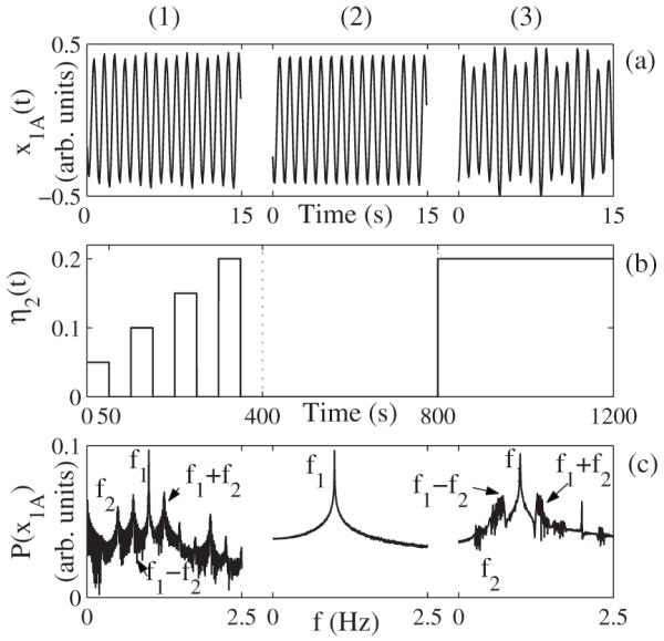
Simulation results for a pair of quadratically coupled Poincaré oscillators in the presence of additive Gaussian noise. (a) The test signal x_1A(t) from the first oscillator, after normalization and subtraction of its mean value. The first oscillator has a characteristic frequency f₁=1.0 Hz. That of the second oscillator is f₂=0.25 Hz. The oscillators are unidirectionally and quadratically coupled with three different coupling strengths η₂(t) in each (1)-(3) 400 s time epoch, shown in (b) as a function of time. In epoch (3) the characteristic frequency of the second oscillator is linearly increased from f₂=0.25 Hz to f₂=0.35 Hz while being at the same time modulated with A_m sin(2πf_mt), where A_m=6.7·10⁻⁶ is the modulation amplitude and f_m=0.01 Hz is the modulation frequency, as can be seen in Fig. 2(b). Each coupling lasts for 400 s. The sampling frequency f_s=10 Hz. Only the first 15 s are shown in each case. (c) The corresponding power spectra of x_1A(t).

FIG. 2.

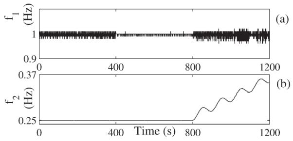
Instantaneous frequencies of (a) the first oscillator f₁ and (b) the second oscillator f₂ in the signal x_1A and x_2A.

1. Bispectral analysis

A quadratic nonlinear interaction between linear or weakly nonlinear oscillatory systems generates higher harmonic components in addition to their characteristic, basic frequencies [20,33]. Figure 1(c) illustrates the changes in the power spectra caused by the coupling. The peaks at f₁=1.0 Hz and f₂=0.25 Hz correspond to the first and second oscillators, respectively. These frequencies are deliberately chosen to have an integer ratio 1:4 to ensure frequency coupling. The test signal x_1A clearly has richer harmonic structure in the presence of nonlinear coupling. In addition to the characteristic frequency of the first oscillator, it contains components with frequencies 2f₁, 2f₂, f₁+f₂, and f₁−f₂. As well as having a particular harmonic structure, the components of the signal x_1A also have related phases, 2𝜙₁, 2𝜙₂, 𝜙₁+𝜙₂, and 𝜙₁−𝜙₂.

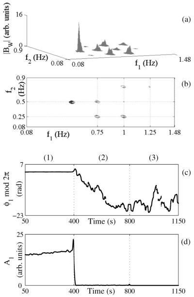
The wavelet bispectrum was calculated from the whole signal as a single entity, after transients caused by the changes in coupling strength had been removed. First the WB was estimated, as shown in Figs. 3(a) and 3(b). Close inspection shows that all the peaks expected to arise from bispectral analysis of nonlinear interaction between the two oscillators f₁ and f₂ are indeed present. Quadratic coupling and how to detect it has already been discussed in detail in [17] and is not a subject of this paper.

FIG. 3.

(a) The modulus of the wavelet bispectrum |B_W| calculated for K=34 segments, 85% overlapping, with T_m=8 s, G_e=0.00001, using a fixed Morlet wavelet length of T_HF=20 s for calculation of the high frequencies. (b) A contour plot of the |B_W|. For f₂>0.9 Hz, the wavelet bispectrum is removed because the triplet (1 Hz, 1 Hz, 1 Hz) produces a high peak that is not physically significant. (c) The biphase 𝜙₁ and (d) the biamplitude A₁ for the bifrequency (1 Hz, 0.25 Hz)-peak 1, calculated using a 0.1 s time step.

Bifrequencies where peaks provide evidence of possible frequency interactions are then further studied by calculation of the biphase and biamplitude as functions of time. The instantaneous frequencies f₁(t) and f₂(t) [Figs. 2(a) and 2(b)] were both obtained using the marked-events method; alternatively they could have been calculated using Hilbert transformation as discussed in detail in [21]. Diagonal elongation of peaks in the bispectrum demonstrates time-variability of the corresponding frequency components.

Our primary interest lies in the bifrequency (f₁, f₂). The time evolution of its biphase and biamplitude are shown in Figs. 3(c) and 3(d). The results for nonzero coupling are remarkably different from those where coupling is absent (intermittent in the first 400 s and during the whole second 400 s). The coupling period can be clearly seen from biamplitude and biphase time evolution in the first 400 s. The biphase is constant in the presence of quadratic coupling (first 400 s) and the biamplitude is above zero. In the first 400 s, each time the coupling strength η₂ is gradually increased, a distinguishable increase in the linear biamplitude value can be noticed.

During the second 400 s there is no coupling as the biamplitude is zero (below-average biamplitude value in the inner triangle [17]) and the biphase is linearly increasing.

During the final 400 s when there is a large time-frequency variation of the second oscillator’s frequency, f₂, which varies within 0.25–0.35 Hz, the biphase is constant and the biamplitude value is high, as shown in Figs. 3(c) and 3(d), and the coupling can easily be resolved.

2. Information theoretic approach

For the same signals in Fig. 1(a) the phases 𝜙₁(t) and 𝜙₂(t) were obtained using the discrete Hilbert transform, and the CMI I[𝜙₁(t) ; Δ_τ𝜙₂ | 𝜙₂(t)] and I[𝜙₂(t) ; Δ_τ𝜙₁ | 𝜙₁(t)] were applied with Δ_τ𝜙_1,2 according to Eq. (17), unless stated otherwise. In order to infer the direction of coupling, we compare the CMI obtained from original data (black) with the CMI calculated from the surrogate data (gray), as shown in Fig. 4. In Fig. 4(a), we can see the influence of the second oscillator, as presented by its time-series x_2A, on the evolution of the first oscillator, presented by time-series x_1A. The opposite influence, i.e., x_1A→x_2A, is depicted in Fig. 4(b).

FIG. 4.

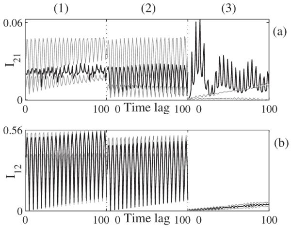
(a) Conditional mutual information (CMI) as a function of time lag (black) together with the surrogate ranges given by the surrogate mean ±1.96σ (gray) from 30 permutation surrogate realizations. (1) denotes intermittent coupling, (2) no coupling and (3) coupling where the characteristic frequency of the second oscillator, f₂, is linearly increasing and being at the same time modulated. (a) The CMI influences 2→1 and (b), the CMI influences 1→2. Lags are from 1 to 100 and 8 quantized levels are used for CMI estimation.

Let us now concentrate on interactions in the three segments, (1), (2), and (3), with different type of couplings. As shown in Fig. 4(a), for segment (3), the CMI is clearly above the surrogate range, i.e., the second oscillator influences the first one. The opposite CMI, as shown in Fig. 4(b), segment (3), is within the surrogates, i.e., there is no influence in the direction x_1A→x_2A. Thus in the case of variable basic frequency the causality is inferred correctly. The same holds for the segment (2): in both cases the CMI lies within the surrogate range, i.e., there is no interaction in any direction, again in agreement with the reality.

Using phases with Δ_τ𝜙_1,2 according to Eq. (17) we obtain misleading results for the first 400 s. In Fig. 4, segment (1), we see that CMI does not cross the surrogate ranges. Here in fact the interaction exists, but we cannot get it from the phases in this way, probably because they are 1:4 locked. Using a synchrogram (not shown) we obtain phase synchronization between the two interacting oscillators. This is the case when phases do not bear information about the causality and, therefore, the direction of coupling cannot be inferred [14].

However, using the phase increment according to Eq. (18) in CMI I[𝜙₁(t) ; Δ_τ𝜙₂(t) | 𝜙₂(t)] and I[𝜙₂(t) ; Δ_τ𝜙₁(t) | 𝜙₁(t)], we have a more sensitive measure. Results for the first 400 s are shown in Fig. 5. The CMI is clearly above the surrogate range in the case when the second oscillator influences the first one, Fig. 5(a), whereas the opposite CMI is within the surrogates, Fig. 5(b). In spite of the presence of phase synchronization and intermittent coupling the causality is inferred correctly.

FIG. 5.

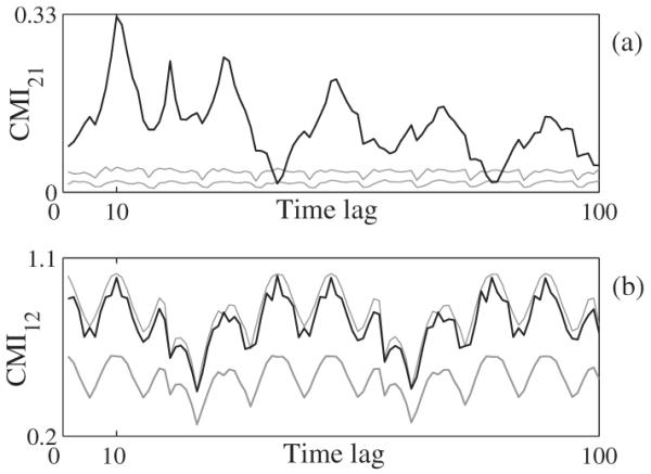
(a) The CMI as a function of time lag (black) together with the surrogate ranges given by the surrogate mean ±1.96σ (gray) from 30 permutation surrogate realizations. For case (1), Fig. 4, the CMI is applied here with Δ_τ𝜙_1,2 according to Eq. (18).

B. Opposite coupling direction and modulation

To illustrate the essence of the method, we again use a generic model of two interacting systems whose basic unit is the Poincaré oscillator

$$\begin{array}{c}\hfill {\stackrel{.}{x}}_1=-x_1{q}_1-({\omega }_1+{\eta }_m{x}_2)y_1+{\eta }_2{(x_1-x_2)}^2+\xi \left(t\right),\hfill \\ \hfill {\stackrel{.}{y}}_1=-y_1{q}_1+({\omega }_1+{\eta }_m{y}_2)x_1+{\eta }_2{(y_1-y_2)}^2,\hfill \\ \hfill {\stackrel{.}{x}}_2=-x_2{q}_2-{\omega }_2{y}_2+{\eta }_1{(x_2-x_1)}^2,\hfill \\ \hfill {\stackrel{.}{y}}_2=-y_2{q}_2+{\omega }_2{x}_2+{\eta }_1{(y_2-y_1)}^2,\hfill \\ \hfill q_i={\alpha }_i(\sqrt{x_i^2+y_i^2}-a_i).\hfill \end{array}$$ (20)

The activity of each subsystem is described by the two state variables, x_i and y_i, where i=1, 2 denotes the subsystem, α_i, a_i, and ω_i are constants, η_1,2 is the coupling amplitude and η_m is the strength of parametric frequency modulation. The parameters of the model are set to α₁=1, a₁=0.5, and α₂, a₂=1, the same as in the case considered in Sec. III A. Here ζ(t) is zero-mean white Gaussian noise ζ(t)=0, ζ(t), ζ(0)=Dδ(t) and D=0.08 is the noise intensity.

The time-series is the variable x_1B(t) of the first oscillator, as shown in Fig. 6(a). Prior to analysis, the signal was first normalized between 0 and 1 and its mean value was subtracted. In the first 400 s the coupling is unidirectional, the second oscillator is forcing the first one with the coupling strength η₂=0.2. After a further 400 s, the forcing was removed by setting η₂=0 and switching on frequency modulation of the first oscillator f₁=1.0 Hz by the second one f₁=0.25 Hz with parametric frequency coupling, η_m=0.1. During the last 400 s, the frequency modulation is removed by setting η_m=0, whereas unidirectional quadratic coupling is present and the coupling direction is reversed. The first oscillator is forcing the second one with the coupling strength η₁=0.2, Fig. 6(b). The first 15 s of each of the three coupling modes is shown in Figs. 6(a), with the corresponding power spectra shown in Fig. 6(c).

FIG. 6.

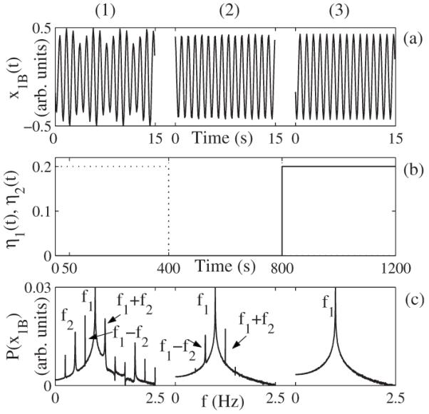
Simulation results for a pair of quadratically coupled Poincaré oscillators in the presence of additive Gaussian noise. (a) The time-series x_1B(t) from the first oscillator, after normalization and subtraction of its mean value. The first oscillator has a characteristic frequency f₁=1.0 Hz. That of the second oscillator is f₂=0.25 Hz. The oscillators are unidirectionally and quadratically coupled with three different coupling strengths η₁ and η₂ in each (1)-(3) 400 s time epoch, both shown on (b) as a function of time, where the solid line represents η₁ and the dotted line η₂. In column (2) the first oscillator is frequency modulated by the second one, η_m=0.1. Each coupling lasts for 400 s. The sampling frequency f_s=10 Hz. Only the first 15 s are shown in each case. (c) The corresponding power spectra of x_1B(t).

Complementary analysis

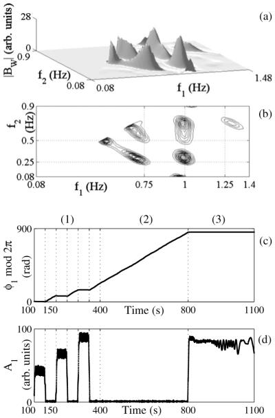
We start with the bispectral analysis. The whole signal x_1B is again analyzed as a single entity, as in the case of test signal 1, x_1A. Auto-WB is shown in Figs. 7(a) and 7(b). Instantaneous biphase and biamplitude for bifrequency (f₁, f₂) are shown in Figs. 7(c) and 7(d). From the constant biphase and above zero biamplitude during the first 400 s we can conclude that nonlinear coupling is present only during first 400 s.

FIG. 7.

(a) The modulus of the wavelet bispectrum |B_W| calculated for K=34 segments, 67% overlapping, with T_m=8 s, G_e=0.00001, using a fixed Morlet wavelet length of T_HF=20 s for calculation of the high frequencies. (b) A contour plot of the |B_W|. For f₂>0.9 Hz, the wavelet bispectrum is removed because the triplet (1 Hz, 1 Hz, 1 Hz) produces a high peak that is not physically significant. (c) The biphase 𝜙₁ and (d) the biamplitude A₁ for the bifrequency (1 Hz, 0.25 Hz)-peak 1, calculated using a 0.1 s time step.

We then applied CMI to the oscillator phases. Obtained results are shown in Fig. 8. During the second 400 s (2), the second oscillator x_2B influences the first oscillator x_1B Fig. 8(a), whereas during the third 400 s (3), the first oscillator drives the second one [Fig. 8(b)], as the CMI is outside the surrogate range.

FIG. 8.

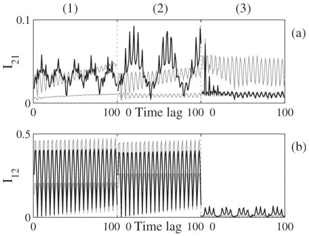
(a) CMI as a function of time lag (black) together with the surrogate ranges given by the surrogate mean ±1.96σ (gray) from 30 permutation surrogate realizations. (1) denotes unidirectional coupling, where the second oscillator drives the first one, (2) where the first oscillator is frequency-modulated by the second one, and (3) denotes unidirectional coupling, where the first oscillator drives the second one. (a) CMI influence 2→1. (b) CMI influence 1→2. Lags are from 1 to 100 and 8 quant levels are used for CMI estimation. For (3) (a) y axis values are multiplied by 100.

The information theoretic approach gives us the correct results for the directionality of interoscillator interactions, whereas it cannot resolve the nature of the interaction. In the second 400 s interval (2), parametric frequency modulation of the first oscillator by the second one is present. CMI cannot distinguish between modulation and nonlinear interaction. To gain additional driver-response information we apply bispectral analysis.

First we calculate the cross-wavelet bispectrum B_Wc121, where the index c stands for cross and the 1, 2 denote state variables of the first and the second oscillators, i.e., x_1B and x_2B, that were used for B_Wc calculation, shown in Figs. 9(a) and 9(b). The x_1B signal tells us primarily about the activity of the first oscillator and x_2B about the second one. The phase of the first oscillator, f₁, in the triplet (f₁, f₂, f₁+f₂) is thus directly extracted from the x_1B signal. Similarly extracted are the phase of the second oscillator and the component at the harmonically related position f₁+f₂. Nonlinear coupling is still present meaning that the second oscillator is driving the first one. One can also verify the results by calculating B_Wc122 (not shown). If the second oscillator is the driver, the nonlinear coupling is no longer present as the third component in the triplet, f₁+f₂. Likewise, it is not present in the signal x_2B, but only in the driven one x_1B. WB_C121 for the last 400 s shows no interaction as the biamplitude is zero and the biphase is not constant, as expected, Figs. 9(a) and 9(b). Note that for the second 400 s the biamplitude is above zero and the biphase is constant. Since auto-WB does not show any interaction during this interval we can conclude that the second oscillator is modulating the first one during the second 400 s. See [17] for further details regarding the detection of parametric frequency modulation.

FIG. 9.

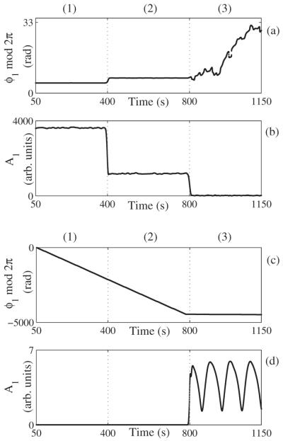
The cross-wavelet bispectrum instantaneous biphase 𝜙₁ and instantaneous biamplitude A₁ for bifrequency (1 Hz, 0.25 Hz)-peak 1, calculated with K=34 segments, 67% overlapping, T_m=8 s, G_e=0.001 and using fixed Morlet wavelet length of T_HF=40 s for high frequencies calculation using a 0.1 s time step. (a) and (b) are for the case of B_Wc121 and (c) and (d) are for the case of B_Wc222.

Similarly we can proceed to identify the reverse interaction, from the first oscillator to the second one. First we calculate the auto-WB, B_Wc222. The biphase and biamplitude are shown in Figs. 9(c) and 9(d). Constant biphase and above-zero biamplitude, in addition to the distinctive position of the peaks in WB [17], demonstrates nonlinear coupling during the last 400 s. This can be verified by further calculation of B_Wc212 and B_Wc211, however it is not necessary due to symmetric properties of the bispectrum [33]. We can determine that the first oscillator is driving the second one during the last 400 s.

IV. SUMMARY AND CONCLUSIONS

In conclusion, wavelet bispectral analysis and information theory approach were combined to investigate the reliability of detection of the nature, strength and direction of coupling of interacting oscillators whose basic frequencies are time-varying. The Poincaré oscillator was used as a generic model.

We generated two distinct numerical examples. With the first, we mimiced typical situations that occur in real measured data, i.e., temporal coupling, time variable strength of coupling and time variable basic frequency. It was shown that by using wavelet bispectral analysis it is possible to resolve the nature and strength of the coupling, even when there are considerable time variations of the basic frequency. Moreover, intermittent nonlinear coupling can be accurately detected. This can be achieved by calculating the instantaneous bifrequency and thus tracing the time variations of the oscillator’s characteristic frequencies using a mother wavelet that allows for an optimal time-frequency resolution. It was shown that by applying the information theory approach and calculating the CMI a possible asymmetry in the coupling can be revealed and quantified. We noted that in the case of the oscillators being synchronized the CMI can lead to incorrect inference of causality from experimental bivariate time series. In this case we can attain information from wavelet bispectral analysis to use the proper variable (state variable, phase, phase increment…) for the CMI calculation to obtain the correct results.

With the second numerically generated example and the corresponding signal x_1B we reversed the coupling direction, the driver and the driven oscillator, adding frequency modulation to mimic one of the most frequent mechanisms of interaction extracted from real measured data. The CMI resolves the correct coupling direction. For the first 800 s the second oscillator drove the first one and for the third 400 s it was vice versa. During the second 400 s frequency modulation was present. We used bispectral analysis to identify it, as with the CMI we cannot attain the answer regarding the nature of the coupling. Moreover, using cross bispectral estimates it was also possible to identify the directionality of coupling by determining the phase origin in the triplet. In this way we could additionally verify the CMI results. We suggest the use of a complementary approach using wavelet bispectral analysis and information theory. The former can resolve the nature and the strength of the coupling, whereas the latter provides reliable information regarding the coupling direction. CMI estimates do not provide the necessary time dependance of the driver response. This can be insufficient when investigating real systems and their coupling dynamics. For this purpose we suggest using the complementary wavelet bispectral analysis where time (and frequency) resolution can be arbitrary set regarding the system dynamics.

The task of revealing coupling dynamics is quite general for any system of coupled nonlinear oscillators where bivariate data can be obtained. It is a highly relevant problem in numerous fields of research, e.g., cardiorespiratory interactions, brain oscillations, neuronal systems, electronic systems, coupled lasers, chemical reactions, to mention only a few. The proposed complementary analysis therefore provides a promising general-use tool for studying the nature, strength and direction of coupling between two (or more) nonlinear oscillators whose basic frequencies considerably change in time.

References

- [1].Hauptmann C, Omel’chenko O, Popovych OV, Maistrenko Y, Tass PA. Phys. Rev. E. 2007;76:066209. doi: 10.1103/PhysRevE.76.066209. [DOI] [PubMed] [Google Scholar]; Kano T, Kinoshita S. ibid. 2008;78:056210. doi: 10.1103/PhysRevE.78.056210. [DOI] [PubMed] [Google Scholar]
- [2].Shiogai Y, Stefanovska A, McClintock PVE. Phys. Rep. 2010;488:51. doi: 10.1016/j.physrep.2009.12.003. [DOI] [PMC free article] [PubMed] [Google Scholar]
- [3].Strogatz SH, Abrams DM, McRobie A, Eckhardt B, Ott E. Nature (London) 2005;438:43. doi: 10.1038/43843a. [DOI] [PubMed] [Google Scholar]; Nakamura S, Kawasaki T. J. Constr. Steel Res. 2006;62:1148. [Google Scholar]
- [4].Ermentrout GB, Rinzel J. Am. J. Physiol. 1984;246:R102. doi: 10.1152/ajpregu.1984.246.1.R102. [DOI] [PubMed] [Google Scholar]; Mirollo RE, Strogatz SH. SIAM J. Appl. Math. 1990;50:1645. [Google Scholar]; Kim D. Biosystems. 2004;76:7. [Google Scholar]
- [5].Schäfer C, Rosenblum MG, Kurths J, Abel H-H. Nature (London) 1998;392:239. doi: 10.1038/32567. [DOI] [PubMed] [Google Scholar]
- [6].Stefanovska A, Bračič M. Contemp. Phys. 1999;40:31. [Google Scholar]; Smelyanskiy VN, Luchinsky DG, Stefanovska A, McClintock PVE. Phys. Rev. Lett. 2005;94:098101. doi: 10.1103/PhysRevLett.94.098101. [DOI] [PubMed] [Google Scholar]; Bahraminasab A, Kenwright D, Stefanovska A, Ghasemi F, McClintock PVE. IET Syst. Biol. 2008;2:48. doi: 10.1049/iet-syb:20060087. [DOI] [PMC free article] [PubMed] [Google Scholar]; Kenwright DA, Bahraminasab A, Stefanovska A, McClintock PVE. Eur. Phys. J. B. 2008;65:425. doi: 10.1140/epjb/e2008-00199-4. [DOI] [PMC free article] [PubMed] [Google Scholar]
- [7].Kryukov AK, Osipov GV, Polovinkin AV, Kurths J. Phys. Rev. E. 2009;79:046209. doi: 10.1103/PhysRevE.79.046209. [DOI] [PubMed] [Google Scholar]
- [8].Hirota M, Tatsuno T, Yoshida Z. Phys. Plasmas. 2005;12:012107. [Google Scholar]; Fukuyama T, Kozakov R, Testrich H, Wilke C. Phys. Rev. Lett. 2006;96:024101. doi: 10.1103/PhysRevLett.96.024101. [DOI] [PubMed] [Google Scholar]; Hartmann P, Kalman GJ, Golden KI, Donko Z. J. Phys. A. 2009;42:214018. [Google Scholar]
- [9].Yao AM, Keen SAJ, Burnham DR, Leach J, Di Leonardo R, McGloin D, Padgett MJ. New J. Phys. 2009;11:053007. [Google Scholar]
- [10].Lam WS, Guzdar PN, Roy R. Phys. Rev. E. 2003;67:025604(R). doi: 10.1103/PhysRevE.67.025604. [DOI] [PubMed] [Google Scholar]; Glova AF. Quantum Electron. 2003;33:283. [Google Scholar]; DeShazer DJ, Breban R, Ott E, Roy R. Int. J. Bifurcation Chaos Appl. Sci. Eng. 2004;14:3205. [Google Scholar]
- [11].Breban R, Ott E. Phys. Rev. E. 2002;65:056219. doi: 10.1103/PhysRevE.65.056219. [DOI] [PubMed] [Google Scholar]; Restrepo JG, Ott E, Hunt BR. ibid. 2005;71:036151. doi: 10.1103/PhysRevE.71.036151. [DOI] [PubMed] [Google Scholar]; So P, Cotton BC, Barreto E. Chaos. 2008;18:037114. doi: 10.1063/1.2979693. [DOI] [PubMed] [Google Scholar]; El-Nashar HF, Muruganandam P, Ferreira FF, Cerdeira HA. ibid. 2009;19:013103. doi: 10.1063/1.3056047. [DOI] [PubMed] [Google Scholar]
- [12].Pikovsky AS, Rosenblum MG, Kurths J. Synchronization; A Universal Concept in Nonlinear Sciences. Cambridge University Press; Cambridge, England: 2001. [Google Scholar]; Pikovsky AS, Rosenblum MG. Physica D. 2009;238:27. [Google Scholar]
- [13].Schreiber T. Phys. Rev. Lett. 2000;85:461. doi: 10.1103/PhysRevLett.85.461. [DOI] [PubMed] [Google Scholar]; Janson NB, Balanov AG, Anishchenko VS, McClintock PVE. Phys. Rev. E. 2002;65:036211. doi: 10.1103/PhysRevE.65.036211. [DOI] [PubMed] [Google Scholar]; Mrowka R, Cimponeriu L, Patzak A, Rosenblum MG. Am. J. Physiol. Regulatory Integrative Comp. Physiol. 2003;285:R1395. doi: 10.1152/ajpregu.00373.2003. [DOI] [PubMed] [Google Scholar]; Bahraminasab A, Ghasemi F, Stefanovska A, McClintock PVE, Kantz H. Phys. Rev. Lett. 2008;100:084101. doi: 10.1103/PhysRevLett.100.084101. [DOI] [PubMed] [Google Scholar]; Schelter B, Winterhalder M, Dahlhaus R, Kurths J, Timmer J. ibid. 2006;96:208103. doi: 10.1103/PhysRevLett.96.208103. [DOI] [PubMed] [Google Scholar]
- [14].Paluš M, Komárek V, Hrnčíř Z, Štěrbová K. Phys. Rev. E. 2001;63:046211. doi: 10.1103/PhysRevE.63.046211. [DOI] [PubMed] [Google Scholar]
- [15].Rosenblum MG, Pikovsky AS. Phys. Rev. E. 2001;64:045202(R). doi: 10.1103/PhysRevE.64.045202. [DOI] [PubMed] [Google Scholar]
- [16].Rosenblum MG, Cimponeriu L, Bezerianos A, Patzak A, Mrowka R. Phys. Rev. E. 2002;65:041909. doi: 10.1103/PhysRevE.65.041909. [DOI] [PubMed] [Google Scholar]; Bezruchko B, Ponomarenko V, Rosenblum MG, Pikovsky AS. Chaos. 2003;13:179. doi: 10.1063/1.1518425. [DOI] [PubMed] [Google Scholar]; Smirnov DA, Andrzejak RG. Phys. Rev. E. 2005;71:036207. doi: 10.1103/PhysRevE.71.036207. [DOI] [PubMed] [Google Scholar]; Kralemann B, Cimponeriu L, Rosenblum MG, Pikovsky AS, Mrowka R. ibid. 2008;77:066205. doi: 10.1103/PhysRevE.77.066205. [DOI] [PubMed] [Google Scholar]
- [17].Jamšek J, Stefanovska A, McClintock PVE, Khovanov IA. Phys. Rev. E. 2003;68:016201. doi: 10.1103/PhysRevE.68.016201. [DOI] [PubMed] [Google Scholar]
- [18].Musizza B, Stefanovska A, McClintock PVE, Paluš M, Petrovčič J, Ribarič S, Bajrovič FF. J. Physiol. 2007;580:315. doi: 10.1113/jphysiol.2006.126748. [DOI] [PMC free article] [PubMed] [Google Scholar]
- [19].Gans F, Schumann AY, Kantelhardt JW, Penzel T, Fietze I. Phys. Rev. Lett. 2009;102:098701. doi: 10.1103/PhysRevLett.102.098701. [DOI] [PubMed] [Google Scholar]
- [20].Jamšek J, Stefanovska A, McClintock PVE. Phys. Med. Biol. 2004;49:4407. doi: 10.1088/0031-9155/49/18/015. [DOI] [PubMed] [Google Scholar]
- [21].Jamšek J, Stefanovska A, McClintock PVE. Phys. Rev. E. 2007;76:046221. doi: 10.1103/PhysRevE.76.046221. [DOI] [PubMed] [Google Scholar]
- [22].Paluš M, Stefanovska A. Phys. Rev. E. 2003;67:055201(R). doi: 10.1103/PhysRevE.67.055201. [DOI] [PubMed] [Google Scholar]
- [23].Hlaváčková-Schindler K, Paluš M, Vejmelka M, Bhattacharya J. Phys. Rep. 2007;441:1. [Google Scholar]
- [24].Nadi AK. Higher-Order Statistics in Signal Processing. Cambridge University Press; Cambridge: 1998. [Google Scholar]
- [25].Kaiser G. A Friendly Guide to Wavelets. Birkhäuser; Boston: 1994. [Google Scholar]
- [26].Proakis JG, Manolakis DG. Digital Signal Processing. 4th ed. Prentice-Hall; New Jersey: 2006. [Google Scholar]
- [27].Bračič M, Stefanovska A. Bull. Math. Biol. 1998;60:919. doi: 10.1006/bulm.1998.0047. [DOI] [PubMed] [Google Scholar]
- [28].van Milligen B. Ph., Hidalgo C, Sánchez E. Phys. Rev. Lett. 1995;74:395. doi: 10.1103/PhysRevLett.74.395. [DOI] [PubMed] [Google Scholar]; van Milligen B. Ph., Sánchez E, Estrada T, Hidalgo C, Branas B, Carreras B, Garcia L. Phys. Plasmas. 1995;2:3017. [Google Scholar]
- [29].Granger CWJ. Econometrica. 1969;37:424. [Google Scholar]
- [30].Cover TM, Thomas JA. Elements of Information Theory. Wiley-Interscience; New York: 1991. [Google Scholar]
- [31].Paluš M, Vejmelka M. Phys. Rev. E. 2007;75:056211. doi: 10.1103/PhysRevE.75.056211. [DOI] [PubMed] [Google Scholar]; Vejmelka M, Paluš M. ibid. 2008;77:026214. doi: 10.1103/PhysRevE.77.026214. [DOI] [PubMed] [Google Scholar]
- [32].Le Van Quyen M, Foucher J, Lachaux JP, Rodriguez E, Lutz A, Martinerie J, Varela FJ. J. Neurosci. Methods. 2001;111:83. doi: 10.1016/s0165-0270(01)00372-7. [DOI] [PubMed] [Google Scholar]; Harrop JD, Taraskin SN, Elliott SR. Phys. Rev. E. 2002;66:026703. doi: 10.1103/PhysRevE.66.026703. [DOI] [PubMed] [Google Scholar]; Quiroga RQ, Kraskov A, Kreuz T, Grassberger P. ibid. 2002;65:041903. doi: 10.1103/PhysRevE.65.041903. [DOI] [PubMed] [Google Scholar]
- [33].Nikias CL, Petropulu AP. Higher-Order Spectra Analysis: A Nonlinear Signal Processing Framework. Prentice-Hall; Englewood Cliffs: 1993. [Google Scholar]