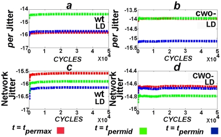
Figure 2. CWO dampens molecule and network jitters in LD.
To avoid the complications of numerical integration over long periods, the integration of these experiments is performed from 0 to 24 hr while computing measurements only at two fixed time points,  and 24 hr;
  corresponds to either the time of the peak (
 ), trough (
 ) of each direct target gene or
  . The procedure is then repeated with the last vector of the previous cycle as initial condition. The numerical integration methods are based on an explicit Runge-Kutta formula, the Dormand-Prince pair (ode45, Matlab), and on a variable order solver based on the numerical differentiation formulas (ode15s, Matlab). Relative error tolerance is
  . Data from ode45 are shown here, the results from ode15s are shown in Figure S4. (a) and (b) plot the jitter of per at
  in the wt and cwo-mutant models in LD, respectively (see Equation 3). (c) and (d) plot the network jitter of the wt and cwo-mutant models in LD, respectively. Notice that the limits converge and that per and network jitters are larger in the cwo-mutant model as compared to wt. Similarly, tim, cwo, pdp1 and vri jitters are also larger in the cwo-mutant models as compared to wt (Figures S1, S2, and S3). Network jitter is lower in the presence of CWO at
  , where
  refers to direct target genes. These times include ZT = 2.91, 4.19, 4.22, 5.2, 5.22, 8.68, 10.07, 10.15, 10.8, 10.99, 14.44, 15.95, 16.4, 16.77 and 19.09 in the wt model and ZT = 6.42, 7.58, 7.88, 7.94, 8.98, 12.19, 13.31, 13.75, 13.76, 14.97, 17.96, 19.04, 19.623, 19.57 and 20.97 in the cwo-mutant model (see Figures S1, S2, and S3).

