Figure 4.

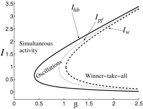
Dynamical regimes in system (2.1) as inhibition strength β and stimulus strength I vary (other parameters are fixed: g = 0.5, τ = 100, r = 10, θ = 0.2). To the left of curve I_hb (solid line) the system has a unique stable equilibrium, and this satisfies u₁ = u₂ (simultaneous activity); in the region between curves I_hb and I_w (dashed line) the system oscillates; then to the right of I_w the system has a winner-take-all behavior (two stable and one unstable equilibria). The curve I_pf (dotted line) indicates a transition from one equilibrium to multiple equilibria in (2.1). While the attractor’s type (limit cycle) does not change between I_hb and I_w, the number of equilibria does: we find one unstable equilibrium between I_hb, I_pf and three unstable equilibria between I_pf, I_w. The turning points of curves I_hb, I_pf, and I_w are obtained at $\beta =\frac{1+1∕\tau }{S^{\prime }\left(\theta \right)}=0.404$, β = g+1/S’(θ) = 0.9, and β_wta = 1.0387, respectively.