A Measurement Error Approach to Assess the Association between Dietary Diversity, Nutrient Intake, and Mean Probability of Adequacy^,,

Abstract

Collection of dietary intake information requires time-consuming and expensive methods, making it inaccessible to many resource-poor countries. Quantifying the association between simple measures of usual dietary diversity and usual nutrient intake/adequacy would allow inferences to be made about the adequacy of micronutrient intake at the population level for a fraction of the cost. In this study, we used secondary data from a dietary intake study carried out in Bangladesh to assess the association between 3 food group diversity indicators (FGI) and calcium intake; and the association between these same 3 FGI and a composite measure of nutrient adequacy, mean probability of adequacy (MPA). By implementing Fuller’s error-in-the-equation measurement error model (EEM) and simple linear regression (SLR) models, we assessed these associations while accounting for the error in the observed quantities. Significant associations were detected between usual FGI and usual calcium intakes, when the more complex EEM was used. The SLR model detected significant associations between FGI and MPA as well as for variations of these measures, including the best linear unbiased predictor. Through simulation, we support the use of the EEM. In contrast to the EEM, the SLR model does not account for the possible correlation between the measurement errors in the response and predictor. The EEM performs best when the model variables are not complex functions of other variables observed with error (e.g. MPA). When observation days are limited and poor estimates of the within-person variances are obtained, the SLR model tends to be more appropriate.

Introduction

The main goal in dietary assessment studies is to determine whether consumption of foods by a sample of individuals is sufficient to meet the nutrient requirements of the sample. Methods for estimating the prevalence of nutrient adequacy have been proposed (1, 2) and can be implemented when a minimum of 2 daily food intake observations is collected for at least some sample individuals. Although the number of observations needed for each person is low, collecting the information is still costly. Interviewers must be trained to accurately record food and beverage intake and an up-to-date, complete food composition database must be available. In resource-poor countries, all of this can be a challenge. The main objective of this work is to explore whether simple measures of dietary diversity can be used to approximately determine whether a sample of individuals is meeting its intake requirements. We present the statistical methodology that can appropriately be used to carry out this type of analysis.

We used a subset of available data from a quantitative dietary intake survey carried out in Bangladesh among women of reproductive age. The main objective of our analysis was to determine whether simple, individual-level measurements of dietary diversity are good predictors of calcium intake and average nutrient adequacy in this sample of women. To meet the goal of the study and, in general, to describe an analytical framework for similar studies, we propose a regression modeling approach that accounts for potentially correlated measurement error in the response and predictor variable. This modeling approach is often known as Fuller’s error-in-the-equation measurement error model (EEM)⁵ approach in the literature (3). To illustrate the performance of the EEM, we carried out a simulation study.

While many dietary intake studies (including the one we discuss in this work) have the type of data required to fit complex models such as the EEM, it is important to recognize that this is not always the case, particularly for studies carried out in resource-poor countries or at a national level. In many instances, all that is available is a 1-d measurement of each sample person’s food consumption. We investigate how much is lost, in terms of inference about mean probability of adequate micronutrient intake (MPA) ( defined later ), when only 1 d of food and nutrient intake is collected for each person in the study.

Because the associations of interest are between usual dietary diversity and usual nutrient intake (for any 1 nutrient) and usual dietary diversity and usual MPA,⁶ some statistical challenges arose in the analysis. Here, usual (4) is used to denote the long-run average dietary diversity, nutrient intake or MPA for a woman, but usual dietary diversity, usual nutrient intake, and usual MPA are not observable in practice. Thus, we accounted for the measurement error in usual dietary diversity and usual nutrient intake to help ameliorate the bias in the ordinary least squares (OLS) regression coefficient estimate (3).

Methods

Description of data and analysis variables

Study sample.

In the analysis presented, we used the 303 nonpregnant, nonlactating (NPNL) women aged 15–49 y from the original Bangladesh study sample. Of the 303 women, 92 were interviewed on 2 nonconsecutive occasions and their 24-h food consumption was recorded on both days. The remaining 211 women were interviewed once and thus their 24-h food consumption was observed for 1 d only. Daily nutrient intake for each woman was estimated using food composition tables appropriate for Bangladesh (5). Nutrients of interest in this study were vitamin A, vitamin C, thiamin, riboflavin, niacin, vitamin B-6, folate, calcium, iron, and zinc. Our analysis of the Bangladesh data focused specifically on calcium intake and MPA.

Nutrient requirements and probability of adequate nutrient intake.

To determine the adequacy of daily nutrient intake by a sample individual we compared the individual’s daily nutrient intake to the appropriate distribution of requirements. Given gender, age and pregnancy/lactating status information, the distribution of requirements of a nutrient for a sample is assumed to be normal with the mean equal to the Estimated Average Requirement (EAR) and SD equal to:

For most nutrients, an EAR has been estimated for the U.S. and Canada populations and the CV set to 10% (6–10). For calcium, an EAR has not yet been determined and thus the distribution of requirements cannot be characterized. The Adequate Intake (AI) can be used to evaluate the adequacy of calcium intake (6). However, because the AI is not an EAR, any inferences about the adequacy of a woman’s calcium intake are approximate at best (6).

In this study, we used the Dietary Reference Intakes for NPNL women 14–50 y identified by Arimond et al. (11) (see Table A2-1). For iron and zinc, we adjusted the EAR proposed by the WHO/FAO (12) for an assumed level of bioavailability of 5 and 34%, respectively (11).

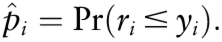
We estimated the probability of adequate daily nutrient intake for a woman by comparing her estimated usual intake to the appropriate distribution of nutrient requirements. Let y_i denote the usual intake of a nutrient by the i^th woman. If r_i denotes requirement of the nutrient for the ^th woman and, r_i ~ N(EAR,(CV × EAR)²), then the probability of AI of the nutrient for the ^th woman in the sample p_i can be estimated as:

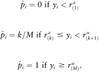
If intakes of a nutrient have been power-transformed, then the distribution of requirements given in the original scale must also be transformed to calculate p_i. A simple approach to estimating p_i in the transformed scale can be implemented as follows. Given a nutrient, draw a large number M of values r₁, …, r_M from a normal distribution with mean equal to the EAR of the nutrient and variance equal to (CV×EAR)². Transform each draw using the same power used to transform observed intakes of the nutrient. If α denotes the power that was used to transform intakes, then r_k^α is the ^th rescaled requirement. Sort the transformed draws in ascending order to obtain the sample order statistics, denoted by r₍₁₎^α,…,r_(M).^α. The probability of adequacy of the daily intake of the nutrient for the woman is then:

where is the estimated probability that the usual intake of a nutrient for woman i is adequate.

The number of draws M must be large enough so that draws from both tails of the distribution are included in the sample. The value of M is arbitrary and in this study, we set M = 1000. This is expected to be large enough across all nutrients to capture nutrient intakes at the lower tail of the distributions as they are bounded by zero.

For iron, the distribution of requirements is assumed to be skewed (9). The appropriate probabilities of AI have been computed for several ranges of usual iron intake and by gender, age group, and pregnancy/lactating status, using a bioavailability assumption of 18% for NPNL women (9). We adjusted these iron intake thresholds to correspond to our assumed iron bioavailability of 5% (11).

Nutrients without an EAR present the greatest challenge when calculating the probability of adequate usual intake for an individual. Calcium is the only nutrient under consideration in this study for which only an AI was available. [Values for AI were obtained from Table A2-2 of (11).] To estimate the probability of adequate daily calcium intake for each woman, we used the approach proposed by Foote et al. (13):

By averaging the estimated probabilities over the ten aforementioned nutrients, we obtain an estimate for MPA.

Food group diversity indicators as a measure of dietary diversity

Several different food group diversity indicators (FGI) were constructed to quantify dietary diversity, varying in level of food group aggregation and minimum consumption required for a food group to count in the FGI score. At the highest level of aggregation, foods were classified into 1 of 6 food groups and at the lowest level of aggregation, foods were classified into 1 of 21 food groups. An intermediate indicator was also constructed by classifying foods into 1 of 13 groups. These 3 levels of aggregation resulted in the FGI known as FGI-6, FGI-13, and FGI-21. The value of each FGI was calculated daily for each woman by counting the number of food groups (in which at least 1 g of food was consumed) included in the woman’s diet. A variant of FGI-6, FGI-13, and FGI-21 was also constructed. These indicators required that at least 15 g of a food be consumed for the food group to count and they are known as FGI-6R, FGI-13R, and FGI-21R (6, 14). The results reported here focus on FGI-13R, FGI-21, and FGI-21R, because these indexes have been identified as more reasonable predictors of nutrient intake and the probability of its adequacy in exploratory analysis.

Description of statistical models

Described in decreasing order of complexity are the statistical methods that can be used to explore the association between FGI and nutrient intake, and FGI and MPA when all variables are subject to measurement error. The different modeling approaches require that different amounts of data be collected on sample individuals. In many resource-poor settings, the more data intensive approaches may not be feasible.

First, the EEM will be described (3). The EEM produces approximately unbiased estimates of the regression slope when the measurement errors on the response and on the predictor variable are correlated. To fit an EEM, estimates of several variances and covariances are required, and thus the method can result in estimators with large SE except in large samples. Also described are less-complex model formulations, including the standard measurement error model (MEM) and simple linear regression (SLR) models when different combinations of data are available for the response and predictor. The MEM assumes that the predictor is observed with measurement error but that the error is uncorrelated to the error in the predicted usual response variable. The SLR model (in all its variations) assumes that the predictor is observable without error.

Y_ij is used to denote the observed response for woman i on day j, and let y_i denote the value of the usual response. In this section, the response might refer to nutrient intake or to MPA, depending on the focus of the analysis.

EEM.

The objective was to assess the association between usual response y_i and usual FGI x_i. If the pair (y_i, x_i) for the ith woman were observable, the SLR model y_i = β₀ + β₁x_i + q_i could be fit, where q_i ∼N(0,σ_qq) for i = 1,…, N and β₁ is the slope of the regression of y_i on x_i. The unobservable usual response for an individual is defined as the long run average of daily responses (at least in some transformed scale); hence, E(Y_ij|i) = y_i for j = 1,…., n_i, Likewise, E(X_ij|i) = x_i, where X_ij is the FGI score for individual i on day j. Under these assumptions, now model daily response (or daily FGI score) as the usual response (or usual FGI score) plus a measurement error for that individual on that day, so that

and

where w_ij and u_ij represent the errors in measuring the usual response and usual FGI score, respectively. Use σ_yy and σ_xx to denote the between-person variances in usual response and usual FGI, respectively, and let w_ij∼N(0,σ_ww) and u_ij∼N(0,σ_uu). Assume (w_ij, u_ij) are independent of q_i and have a bivariate normal distribution:

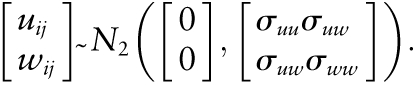Here, σ_ww and σ_uu are the within-person variances in daily response and daily FGI, respectively, and σ_uw is the covariance between the errors in the observed values of the response and predictor variables.

If the hypothesis that β₁ = 0 is rejected, we conclude that there is a linear association between the usual response (either usual nutrient intake or usual MPA) and usual FGI. Thus, to assess the association between usual response and usual FGl, the methods focus on estimating β₁ and its variance. Methods used in estimating the slope and variance components of the EEM can be found in the Supplemental Materials.

Standard MEM.

When it is assumed there are uncorrelated measurement errors between the predictor and response, one can obtain an unbiased estimate of β₁ with the MEM given that can be estimated. Given observations (Y_ij, X_ij), the MEM is

and

where (x_i,q_i,u_i) ∼N[(μ_x,0,0), diag(σ_xx,σ_qqσ_uu)]. Estimation of these model parameters is similar to that of the EEM. Details of this estimation can be found in the Supplemental Materials.

SLR model when at least 2 d of data are available for the predictor and response.

Assuming that the predictor is observed with measurement error that is uncorrelated with the error in the response, an alternative to the MEM is to fit a SLR model to the best linear unbiased predictor (BLUP) of the response and o the predictor (3,14). The BLUP is best in the sense that among all linear unbiased predictors of y_i or x_i, it minimizes the prediction error variance. If σ_yy and σ_ww are known, the BLUP of the usual response (15) is defined as:

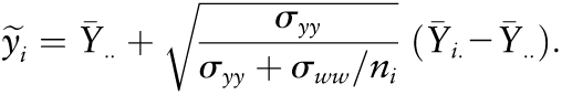Likewise, the BLUP of the usual predictor is

given σ_xx and σ_uu. The BLUP is known as a shrinkage estimator of a variable, because it shrinks the person-level mean for that variable toward the overall group mean. The amount of shrinkage depends on the relative size of the within-person to the between-person variability in the variable. Thus, fitting a SLR model to the BLUP of (y_i, x_i) is approximately the same as fitting the MEM to (Y_ij, X_ij). However, this approach, like the EEM and MEM, requires at least 2 d of data for the predictor and response for at least some individuals in the sample.

SLR model when only 1 d of data is available for the predictor.

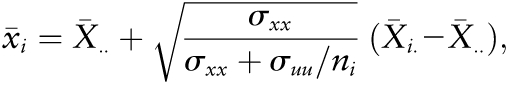
When 2 d of data are not available for both the predictor and response for at least a subsample of individuals, a different SLR approach must be used. If only 1 observation day is available on the predictor, but a reliable estimate of y_i from multiple observation days (perhaps the BLUP) is available, the BLUP of the usual response can be regressed on the observed predictor on d 1 X_i1. If, on the other hand, only 1 observation is available for both the predictor and response for each individual in the sample, then it is only possible to regress the response from d 1 Y_i1 on its corresponding predictor variable from d 1 X_i1.

If it is known that the predictor is observed with measurement error, one must accept that in these 2 SLR approaches, the OLS estimate of the slope will be biased toward 0 or attenuated. An estimate of the attenuation coefficient κ_xx might be available from a different study, and if so the OLS estimate of the slope can be adjusted. An unbiased estimate of the true slope β₁ of the usual response and usual predictor is given by

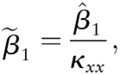where is the OLS estimate for the slope and

To estimate the attenuation coefficient, assume that σ_xx and σ_uu are known. By using both days of data, one can obtain estimates for these variances: and can be estimated from Eq. 2 in the Supplemental Materials. To test the hypothesis that β₁ ≠ 0, we need to estimate the variance of the adjusted estimate of the slope:

where is the mean squared error (MSE) of the SLR model.

Results

Model assessment via simulation

In what follows, the results of a simulation assessing the validity of the SLR model in capturing the linear association between 2 variables where both are observed with error are described. Here, only the EEM and the SLR are compared, but a larger comparison that includes the MEM and the SLR using BLUP could also be implemented if space were not limited. First, pairs (y_i, x_i) are simulated and then correlated measurement errors are added to obtain “observed” pairs (Y_ij, X_ij). By simulating data from a model where measurement error is present and the true association is known, one can evaluate the appropriateness of using the OLS estimator of the slope in this type of problem.

Values of the parameters of the measurement error model were fixed: β₀, β₁, σ_uu, σ_ww, σ_uw, σ_qq, μ_x, and σ_xx, where μ_x is the mean of x_i across all individuals. Parameter values were chosen to be similar to the estimates obtained from the EEM fit to calcium intake and FGI in the Bangladesh data.

To generate n_i simulated daily responses and daily FGI scores for N individuals, the following steps were implemented: 1) generate model errors q_i from N(0,σ_qq) for i = 1,…, N; 2) generate usual FGI values x_i from N(μ_x,σ_xx)for i = 1,…, N; 3) calculate the usual response values y_i, where y_i = β₀ + β₁x₁ + q_i for i = 1,…, N; and 4) generate the “observed” values from

Once the daily responses and predictors were simulated for a given set of initial conditions, both the SLR model and the EEM were fit to the data. This process was repeated 500 times always using the same set of parameter values to generate the simulated data. The means of the 500 slopes and are the estimates of the true slope obtained by the SLR model and EEM, respectively. In each case, the 95% CI for the true slope also can be computed (empirically) from the 500 estimates. If these CI cover the true value of the slope β₁, then with 95% probability, the model produces plausible estimates of the slope. If not, the slope estimate is significantly different from the true slope, suggesting that the model is not appropriate for the data.

Varying the within-person measurement error variance in the predictor.

First, σ_uu was varied and the model error variance and response measurement error variance at σ_qq = 0.05 and σ_ww = 0.3, respectively, were fixed. Fixing the correlation between the measurement errors in the response and the predictor at 0.5 causes the covariance of the measurement errors to vary with the measurement error variances, because

Fixing β₁ = 0.1and β₀ = 30 and choosing several values for the measurement error variance of interest (_σuu = 0.0, 0.6, 1.2, 1.8, 2.4, and 3.0), 500 datasets were simulated with 200 individuals each with n_i = 2 observations using each of the 6 sets of parameter values.

When measurement error in the predictor is absent (i.e. σ_uu = 0), the SLR model and EEM produce similar estimates of β₁ (Fig. 1). Although there is still measurement error in the response variable, it is absorbed by the model error σ_qq under the assumptions of the SLR model. As the variance in the measurement error of the predictor increases, the mean of the OLS slope estimate begins to deviate from the true value of 0.1. For lower measurement error variances of the predictor, this model tends to overestimate the true slope. However, the bias of the OLS estimate decreases as the variance of the predictor increases; eventually, the bias becomes negative and the slope is underestimated. The EEM performs differently. As the variance component increases, the error-adjusted estimates appear unbiased regardless of the size of the within-person variance in the predictor.

FIGURE 1.

Empirical means and 95% CI for the slope β₁ = 0.1 based on 500 simulations for the SLR model and the EEM. The following parameter values were used in the data simulation: β₀ = 30, μ_x = 4, and σ_xx = 1. (A) σ_ww = 0.3 and where σ_uu takes on values 0.0, 0.6, 1.2, 1.8, 2.4, and 3.0. (B) σ_uu = 1 and where σ_ww takes on values 0.0, 0.2, 0.4, 0.6, 0.8, and 1.0. (C) σ_uu = 1 and σ_ww = 0.3, where σ_uw takes on values ranging from

When the SLR model was fit to the simulated data with measurement error, the narrowing width of the 95% CI indicated the variance of the OLS estimate slightly decreased as the σ_uu of the predictor increased. In contrast, and as expected, the width of the CI for the error-corrected estimates of the slope increased appropriately with the increase in measurement error variance.

Varying the within-person measurement error variance in the response.

To further investigate the bias of the OLS estimator for the linear association between 2 variables observed with measurement error, more data were simulated, varying σ_ww, the variance of the measurement error in the response variable. Fixing σ_uu = 1 and allowing σ_ww to take on several values (0.0, 0.2, 0.4, 0.6, 0.8, and 1.0), the same values for all other parameters were used as in the previous case and 500 datasets for each of these sets of parameters were simulated.

When there is no measurement error in the response, σ_ww = 0, the SLR model and EEM perform similarly well in estimating the true slope (Fig. 1). As the σ_ww increases, the bias in the OLS estimator also increases. If the variability in the response increases while the predictor variance remains fixed, the SLR model will produce a slope estimate with a bias that increases (in absolute value) as the response error variance increases. Whether the bias is positive or negative depends on the sign of the estimated slope. Again, the EEM appears to produce unbiased estimates of the true slope for each value of σ_ww.

When using the SLR model on data observed with measurement error, the measurement error in the response now contributes to the overall model error. Thus, the model error variance in the SLR model σ_qq increases with σ_ww, producing wider CI for larger response error variances. In the EEM, the increase in the CI width is attributable to an increasing σ_ww, which results in increased variance of the error-corrected estimate of the slope.

Varying the value of the covariance.

To assess how the magnitude of the covariance affects the OLS estimator, the measurement error variances were fixed and only their covariance varied. For simulation, we used β₀ = 30, β₁ σ_qq = 0.1,σ_ww = 0.3, = 0.1, σ_qq = 0.05, σ_ww = 0.3, and σ_uu = 1. In particular, the measurement error variances chosen are akin to those identified in exploratory analysis. Covariance values that yield measurement error correlations ρ_uw between −1 and 1 were chosen. Hence, results in covariance values ranging from It can be seen that the OLS estimator is biased for the true slope when measurement error is present (Fig. 1). The bias of increases as the absolute value of the correlation between the measurement errors increases. In contrast, the EEM estimator is approximately unbiased.

Although the simulated predictor variables were truly observed with error, by assumption, the SLR model treated them as if they were not. Because predictor error variance was ignored here (i.e. assume σ_uu = 0), the covariance between the “nonexistent” errors must be treated in same way (i.e. assume σ_uw = 0). Therefore, varying σ_uw did not affect the variance of the OLS estimate of the slope, as indicated by the constant width of the CI obtained from the SLR model. In contrast, the CI obtained from the EEM estimates of the slope appeared to decrease slightly in width with increasing covariance. This can be attributed to the quadratic nature of the variance estimate of the error-corrected slope estimate in σ_uw.

Fitting the models to the Bangladesh data

The results obtained from fitting the models to the Bangladesh data are presented here. First, the results from fitting the EEM to calcium intakes are summarized. The MEM and different forms of the SLR model were fit to MPA; however, only results obtained from the SLR model fits are presented.

Because the assumption of normality underlies all of the methods implemented, it is first verified that the response and, where necessary, the predictor were normally distributed, at least after transformation. By visual inspection, FGI tended to be approximately normally distributed across sample individuals. Calcium intakes were skewed to the right in the original scale; therefore, the Box-Cox (16) approach suggests a log transformation, which resulted in an approximately normal distribution of intakes.

To estimate the probability of AI of each nutrient and consequently the MPA for each woman, a log transformation of each micronutrient intake into the (approximately) normal scale was done. Then the BLUP of usual nutrient intake for each woman and each nutrient were obtained and used to compute the probability of AI for each nutrient. The probabilities of adequacy were averaged across the 10 micronutrients of interest to obtain the MPA for each individual in the sample (17). To verify the assumption of normality for MPA, 0.80 was identified as the best power transformation to achieve near normality for MPA given that MPA is a proportion and takes on values between 0 and 1 (Supplemental Fig. 1).

EEM for calcium intakes.

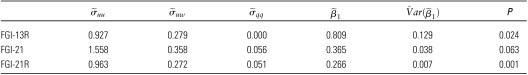
To assess the association between usual FGI and usual calcium intake, the EEM was fit using transformed calcium intake as the response and FGI as the predictor variable. Using Eq. 1, 2, and 3 in the Supplemental Materials, the within-person variances and covariance estimates for the measurement errors in the EEM were computed. The within-person variance estimate of calcium intake was 0.552. The estimates of within-person variances for the FGI increase as more food groups were incorporated into the FGI (Table 1). For example, the variance estimate for FGI-13R, is lower than the variance estimates for FGI-21 (1.558) and FGI-21R (0.963). Within each level of food group aggregation, the more restrictive 15-g minimum consumption criterion yielded a smaller variance across FGI. The covariance estimates all of which were positive, were similar in order of magnitude to the FGI variance estimates.

TABLE 1.

Estimates of parameters in the EEM using usual FGI as a predictor of usual calcium intake

Because the method of moments does not place any constraints on the parameter space, estimates that fall outside of the parameter space are possible. In Eq. 5 of the Supplemental Materials, the estimate for σ_qq is the MSE of the model (s_vv) adjusted for additional variability contributed by the measurement error in the variable (s_rr). The error in the model attributable to measurement error slightly exceeded the MSE of the model, resulting in a negative estimate of the model error variance. In such cases, set the negative estimates of σ_qq to 0, the closest value to the actual estimate contained in the parameter space.

The variance and covariance estimates can be used to adjust the OLS estimates and variances of the slope β₁. After accounting for the measurement error in both the response and the predictor, a positive association was observed between calcium intakes and most FGI at P < 0.05 (Table 1). FGI-13R and FGI-21R resulted in slopes that significantly differed from 0. As the FGI score increased, so did usual calcium intake. The actual magnitude of the slope decreased as more food groups were included in the FGI. This is because in the less aggregated FGI, each food group is likely to contribute a smaller amount of the nutrient. The less aggregated FGI tend to result in more significant associations with calcium intake.

Residual plots were used to assess the fit of the EEM for the calcium model (Supplemental Fig. 2). With FGI-21 and FGI-21R, the Studentized residuals took on acceptable values and did not exhibit a trend in the residual plot. With FGI-13R, however, the residuals exhibited a negative trend, suggesting that FGI-13R alone does not provide enough information about calcium intake.

SLR model for MPA when at least 2 d of data are available for the predictor and response.

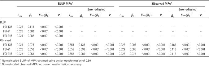
Now presented are results that were obtained by fitting a SLR model to different observed and estimated variables. First, the regression of the BLUP of MPA on the BLUP of FGI was a way of approximating the results that would be obtained from the MEM. (Throughout this section, the BLUP of MPA refers to the MPA calculated using the BLUP of each nutrient intake, not the observed intakes.) A significant positive linear association was demonstrated between the BLUP of MPA and that of FGI (Table 2). The positive slope indicated that as more food groups are consumed, usual MPA is expected to increase as well. FGI-21 and FGI-21R resulted in smaller slopes than FGI-13R. The estimate for the variance of the model error σ_qq differed very little across FGI. The residual plots for each regression had acceptable values and showed no trend (Supplemental Fig. 3); this suggests that fitting a SLR model to the BLUP of FGI as a predictor of usual MPA is reasonable, at least in this study.

TABLE 2.

Estimates of the unknown parameters in the SLR of MPA on FGI and the error-adjusted estimates

SLR model for MPA when only 1 d of data is available for the predictor.

Next, a SLR model was fit that regressed the BLUP of MPA on FGI calculated using only d 1 of food consumption. The OLS estimate of the slope was positive and significant for all FGI (Table 2). Again, the less aggregated FGI resulted in a lower estimate of the slope. The residual variance was very similar for FGI-13R, FGI-21, and FGI-21R. The residual plots for each FGI suggest that the SLR model fit these data well (Supplemental Fig. 4). However, using a 1-d FGI to predict usual MPA via a SLR model resulted in an attenuated estimate of the slope. If an estimate of the attenuation coefficient κ_xx is available, perhaps from other similar studies, it is possible to adjust the OLS estimate of the slope to reduce the bias. The attenuation coefficient estimate for the Bangladesh data varied by FGI, ranging from 0.554 to 0.653 (Table 2). Smaller values of k_xx resulted in greater adjustments. The slope for each FGI was more significant after adjusting for attenuation.

SLR model for MPA when only 1 d of data is available for the predictor and response.

Finally, using only the intake data collected on d 1, observed MPA was regressed on observed FGI. Slope estimates for this model were similar in magnitude to those obtained when the SLR model was fit to the BLUP of MPA and that of FGI (Table 2). Analysis of residuals from fitting the model did not suggest any violation of model assumptions. Using the attenuation coefficient to correct for measurement error nearly doubled the OLS estimate of the slopes and preserved the significance (Table 2).

Discussion

The main contribution of this article is methodological; we argue that via simulation, naive regression modeling and estimation can be inappropriate when both the response and the predictor variable are measured with correlated error. In these cases, it is important to design studies that permit fitting an EEM or at least a MEM. This said, in resource-poor countries, the funds to carry out multiple 24-h recalls with large, representative samples are not always available and consumption information might be limited. Thus, also discussed are approaches to fit less complex models and interpret results appropriately under these simpler models.

Provided is a blueprint for parameter estimation and result interpretation in a wide range of data scenarios. Because the type of intake data and the nature of the underlying research question in this work arise often in nutrition epidemiology and public health, it is anticipated that this contribution will be valuable beyond our particular application.

Assessing the relationship between usual FGI and usual calcium intake and between usual FGI and usual MPA was also an objective of this work. An EEM that accommodates the correlated measurement errors in the daily value of the response and of the predictor is, in principle, the optimal approach. This approach was used to investigate the association between usual FGI and usual calcium intake. When the response variable is in itself a complex function of unobservable quantities, correctly implementing the errors-in-the-equation approach is difficult. This is the case with, e.g., MPA.

An intermediate approach based on a MEM was also described. The MEM accounts for the measurement error in observed FGI but assumes no correlation between this error and the usual noise with which the response variable is observed. When fitting a MEM to MPA, slope estimates were positive but had large SE and were thus not significant (results not shown). This is attributable at least in part to the complex form of the response variable. It appears that for the Bangladeshi data, the MEM produces more reliable results even if they are less attractive than the SLR approach.

To explore the association between a complex function of nutrient intakes (such as MPA) and FGI, a more simple methodology is proposed that can approximate the results that would be obtained from the measurement error approach. The approximate methodology carries out the analysis in 2 steps. First, obtain the BLUP of usual nutrient intake and of the usual FGI for each individual. Second, compute the person-level usual MPA using the predicted usual intakes. Finally, a SLR is carried out, using the BLUP of FGI as the predictor and the BLUP of MPA as the response.

The difference between this 2-step approach and the EEM approach is the 2-step analysis ignores the correlation between the 2 measurement errors (in the response and the predictor). Thus, the inferences drawn from the EEM approach and the approximation we propose here will be similar when the correlation between measurement errors is low and less similar when the correlation is strong.

If data are not available on the response and the predictor for ≥2 d, the 2-step approach above cannot be implemented. However, if an attenuation coefficient is available from another study, the slope estimated from a SLR model can be corrected. These results show that after correcting the OLS slope with the attenuation coefficient estimated with the Bangladesh data, the results for the SLR model begin to approach those obtained from fitting the MEM. This suggests that it might be possible to improve on SLR results in studies where only 1 observation per person may be available if a suitable reliability coefficient k_xx can be “borrowed” from a different study. This approach is similar to what was proposed by Jahns et al. (18).

Significant associations between usual FGI and usual calcium intake were detected by the EEM. It was argued earlier that when the response is a complex function of unobservable variables, as is the case of MPA, uncovering significant associations is more difficult for various reasons. First, measurement error is present in the estimation of each probability of adequacy for the various nutrients. By averaging these probabilities across all 10 nutrients to estimate MPA, we are using a complex function of already-noisy estimates of the probability of adequate nutrient intake, thus decreasing the likelihood of detecting an association between usual FGI and usual MPA. Second, the Bangladesh sample was small and 2 d of information were available for only a small proportion of women. This adds to the uncertainty with which we can estimate variances and covariances and thus the uncertainty in the reliability of the various adjustments that comprise the EEM approach. When one is not confident that good estimates of variances and covariances can be obtained, it might be better to implement a simpler approach.

Considering that FGI are simple in that they tell little about which foods were consumed by an individual and provide limited information about the quantity of food consumed, some FGI performed reasonably well at identifying linear associations with calcium intake. Adjusting the consumption criterion and food group definitions may lead to even more encouraging results. For MPA and FGI, much larger samples might be required to uncover an association using the EEM approach.

Literature Cited

- 1.Beaton GH. Criteria for an adequate diet. Shils ME, Olson JA, Shike M, Modern nutrition in health and disease. 8th ed Philadelphia: Lea & Febiger;1994:1491–505 [Google Scholar]
- 2.Carriquiry AL. Assessing the prevalence of nutrient inadequacy. Public Health Nutr. 1999;2:23–33 [DOI] [PubMed] [Google Scholar]
- 3.Fuller WA. Measurement error models. New York: John Wiley & Sons; 1987 [Google Scholar]
- 4.Nusser SM, Carriquiry AL, Dodd KW, Fuller WA. A semi-parametric transformation approach to estimating usual nutrient intake distributions. J Am Stat Assoc. 1996;91:1440–9 [Google Scholar]
- 5.Arimond M, Wiesmann D, Torheim LE, Joseph M, Carriquiry A. Dietary diversity as a measure of the micronutrient adequacy of women’s diets: results from rural Bangladesh site. Washington, DC: Food and Nutrition Technical Assistance Project II (FANTA-2) at Academy for Educational Development (AED); 2009 [Google Scholar]
- 6.IOM Dietary reference intakes for calcium, phosphorus, magnesium, vitamin D and fluoride. Washington, DC: National Academies Press; 1997 [PubMed] [Google Scholar]
- 7.IOM Dietary reference intakes for thiamin, riboflavin, niacin, vitamin B6, folate, vitamin B12, pantothenic acid, biotin, and choline. Washington, DC: National Academies Press; 1998 [PubMed] [Google Scholar]
- 8.IOM Dietary reference intakes for vitamin C, vitamin E, selenium and carotenoids. Washington, DC: National Academies Press; 2000 [PubMed] [Google Scholar]
- 9.IOM Dietary reference intakes for vitamin A, vitamin K, arsenic, boron, chromium, copper, iodine, iron, manganese, molybdenum, nickel, silicon, vanadium, and zinc. Washington, DC: National Academies Press; 2000 [PubMed] [Google Scholar]
- 10.IOM Dietary reference intakes for energy, carbohydrate, fiber, fat, fatty acids, cholesterol, protein, and amino acids (macronutrients). Washington, DC: National Academies Press; 2002 [DOI] [PubMed] [Google Scholar]
- 11.Arimond M, Wiesmann D, Becquey E, Carriquiry A, Daniels M, Deitchler M, Fanou N, Ferguson E, Joseph M, et al. Simple food group diversity indicators predict micronutrient adequacy of women#x2019s diets in five diverse, resource-poor settings. J Nutr. 2010;140:2059–369 [DOI] [PMC free article] [PubMed] [Google Scholar]
- 12.WHO and FAO Vitamin and mineral requirements in human nutrition. 2nd ed Geneva: WHO; 2004 [Google Scholar]
- 13.Foote JA, Murphy SP, Wilkens LR, Basiotis PP, Carlson A. Dietary variety increases the probability of nutrient adequacy among adults. J Nutr. 2004;134:1779–85 [DOI] [PubMed] [Google Scholar]
- 14.Carroll RJ, Ruppert D, Stefanski LA, Crainiceanu CM. Measurement error in nonlinear models. A modern perspective. 2nd ed New York: Chapman and Hall; 2006 [Google Scholar]
- 15.Henderson CR. Selection index and expected genetic advance. : Hanson WD, Robinson HF, Statistical genetics and plant breeding; A research symposium and workshop; 1961 Mar 20–29, Washington: NAS-NRC; 1963p141–163 [Google Scholar]
- 16.Box GEP, Cox DR. An analysis of transformations. J Royal Stat Soc Series B Stat Methodol. 1964:26:211–246 [Google Scholar]
- 17.Joseph ML. Dietary diversity and probability of nutrient intake adequacy among women in Bangladesh [Masters creative component]. Ames (IA): Iowa State University; 2007 [Google Scholar]
- 18.Jahns L, Arab L, Carriquiry AL, Popkin B. The use of external within-person variance estimates to adjust nutrient intake distributions over time and across populations. Public Health Nutr. 2005;8:69–76 [DOI] [PubMed] [Google Scholar]