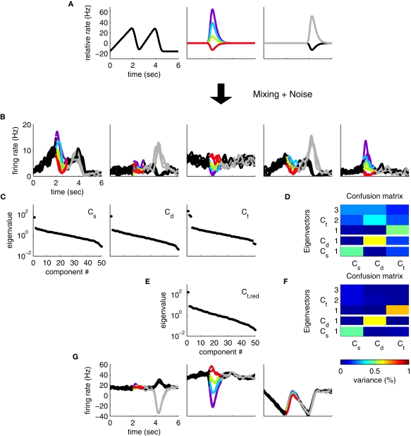
Figure 3.

Heterogeneous responses as a result of linear mixture of three components. (A) We now assume that neural responses are constructed from three underlying components, one of which encodes only the task rhythm (left), while the two others encode stimuli and responses, as in Figure 1. (B) Single cell responses are random combinations of these three components. We again assume that N = 50 neurons have been recorded, five of which are shown here, and response noise was generated as in Figure 1. (C) Whereas the marginalized covariance matrices for stimulus and decision, C_s and C_d, have only one significant eigenvalue, the one for time, C_t, features three eigenvalues above the noise floor. (D) The confusion matrix displays the percentage of variance captured by the different components (y-axis) with respect to the different marginalized covariance matrices (x-axis). The C_s row shows, for instance, that the first eigenvector of C_s captures a significant amount of variance from the C_s matrix (which is good), but it also captures a significant amount of variance from the C_t matrix (which is bad). (E) By estimating the time-dependent covariance over a time window limited to t∈[0,2], we can reduce the number of significant eigenvalues to one. (F) In turn, every row of the confusion matrix has only one entry, showing that every component captures the variance of one marginalized covariance matrix only. (G) The firing rates projected onto the components from (F).