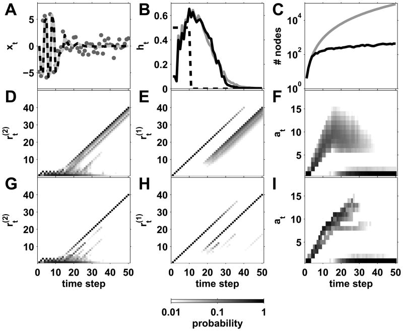
Figure 6.

Effect of pruning on a three-level hierarchy example. A The data (circles) are sampled from a Gaussian distribution whose mean changes every 2 time steps for t ≤ 10 and then remains constant afterwards. The predictive mean is shown for the unpruned (dashed black) and pruned (gray) model. B The model’s estimates of h (gray line unpruned, black line pruned) compared with the generative h (dashed black line). C The number of nodes for the unpruned (gray) and pruned (black) cases over time on a logarithmic scale. D Marginal low-level run-length distribution, $p(r_t^{(2)}\mid x_{1:t})$, in the unpruned case. This is to be compared with the pruned version of the same distribution in panel G. E and H Marginal high-level run-length distribution, $p(r_t^{(1)}\mid x_{1:t})$, in the unpruned and pruned cases respectively. F and I Marginal change-point count distribution, p(a_t|x_1:t), in the unpruned and pruned cases.