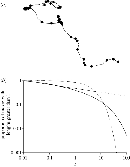
Figure 2.
(a) An example of a simulated movement pattern produced by two independent Langevin equations (σ = 1, T = 10) for the x- or y-components of velocity. The Langevin equations were integrated numerically with a time step Δt = 0.01 arbitrary time units. The turning points where the direction of travel changed by an amount Δθc = 45° are indicated (filled circle). (b) The survival function (the complement of the cumulative distribution) of ‘move’ lengths travelled between consecutive turns (solid line). Shown for comparison are the maximum-likelihood power-law (dashed line) and exponential (dotted line) distributions. A straight line on this log–log plot is indicative of power-law scaling. Here, approximate power-law scaling is seen to extend over about two decades.

