Figure 4. Combinatorial constraints on population firing rate vectors.

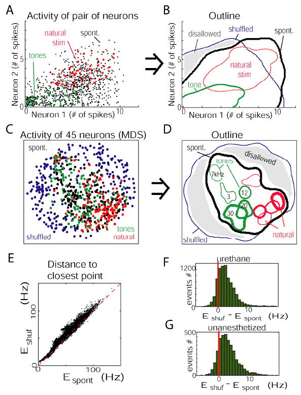
(A) Spike counts of two neurons (recorded from separate tetrodes) during the first 100ms of spontaneous upstates (black), responses to a tone (green), and natural sound (red). Data were jittered to show overlapping points. Note that regions occupied by responses to the sensory stimuli differ, but are both contained in the realm outlined by spontaneous patterns. (B) Contour plot showing regions occupied by points from (A). The blue outline is computed from spike counts shuffled between upstates, indicating the region that would be occupied in the absence of spike count correlations. (C) Firing rate vectors of entire population, visualized using multidimensional scaling; each dot represents the activity of 45 neurons, nonlinearly projected into two-dimensional space. (D) Contour plot derived from multidimensional scaling data, with responses to individual stimuli marked separately. Sensory-evoked responses again lie within the realm outlined by spontaneous events. (E) Scatter plot showing the Euclidean distances from each evoked event to its closest neighbor in the spontaneous events (E_spont), and in the shuffled spontaneous events (E_shuf). Dashed red line shows equality. (F, G) Histogram showing the difference between distances to shuffled and spontaneous events (E_shuf - E_spont). Top and bottom: data from all anesthetized and unanesthetized experiments, respectively. Almost every evoked event was closer to a true spontaneous vector than to a shuffled vector. Adapted from Luczak et al (2009).