Figure 8. Difference in propagation of activity across cortical layers and columns.

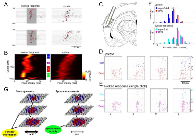
(A) Example laminar profiles of upstates and evoked responses. Rasters indicate MUA of all channels on a 32-site linear probe for individual upstates and evoked responses. Shaded periods indicate tone presentations. Red dots indicate “peak latency,” computed as the median MUA spike time in a 50-ms window after event onset. (B) Laminar profiles of peak latency for tone-evoked responses (best frequency, 60-80 dB SPL) and upstates. The graphs show a pseudocolor histogram of the distribution of peak latency as a function of depth. (C) Two-shank multisite electrodes (2×16 linear probe) were inserted parallel to the layers of auditory cortex. A part of the drawing was replicated from (Paxinos & Watson 1997). (D,E) Examples of spatiotemporal patterns for upstates (D) and click-evoked responses (E). Each plot shows rasters of MUA on all recording sites, with superficial and deep shanks on top and bottom. The sites on each shank are arranged from dorsal (D) to ventral (V). (F) Distribution of propagation speeds for upstates (top) and evoked responses (bottom), estimated as the regression slope of median MUA time across recording sites. Arrows indicate the median, and the x-axis is log-scaled. Propagation speed was faster for evoked responses than for upstates in both layers (ANOVA with post hoc lsd test, p<0.0001). (G) Hypothesized flow of sensory-evoked and spontaneous activity through auditory cortical circuits. Each sheet represents a population of the corresponding layer, with cones and spheres representing PCs and INs, respectively. Colored symbols represent active neurons. Adapted from Sakata and Harris (2009)