Figure 1.

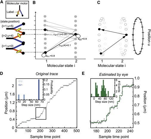
Models of molecular motor activity. (A) A two-state model for a linear molecular motor. The system starts in molecular state i = 1 with its fluorescent label (oval) at position u = 0. After a certain dwell time, the molecule undergoes a conformational change swinging its trailing leg forward, displacing the label by w = 4 units and settling into state 2. Subsequently, the molecule makes a transition back to state 1 with the label making a displacement of w = 1. (B) Two transitions of a Markov model describing the molecule in panel A. Initially, the molecule has a probability of a₁₁ = 0.8 of staying in state 1 with a mean dwell time of 1/(1–0.8) = 5 time units in this state. When the molecule makes a transition to state 2, it can change position with a step of size w = 3, 4, or 5 units; exemplary step of four units in bold (with transition probability c₁₂(4) = 0.1). After a dwell in state 2 (mean dwell of 10 time units), a transition can be taken back to state 1 with size w = 1, 2, or 3 units (step of one unit in bold). (C) The position values are wrapped around into a periodic coordinate system, exploiting the local nature of changes in the motor's position. (D) An example simulation of a molecular motor that moves with alternating short (10 or 20 nm) and long (64 nm) steps. Average dwells after short and long steps are 10 and 5 time points, respectively. Gaussian noise with σ = 7 nm was added to simulate the noisy trace (gray dots). (Inset) Simulated step probabilities c₁₂ and c_21. (E) An enlarged section (box in D) showing details of the time course. A fit by eye (solid line) yields the apparent step size distribution shown in the inset.