Automated image analysis for tracking cargo transport in axons

Abstract

The dynamics of cargo movement in axons encodes crucial information about the underlying regulatory mechanisms of the axonal transport process in neurons, a central problem in understanding many neurodegenerative diseases. Quantitative analysis of cargo dynamics in axons usually includes three steps: (1) acquiring time-lapse image series, (2) localizing individual cargos at each time step, and (3) constructing dynamic trajectories for kinetic analysis. Currently, the later two steps are usually carried out with substantial human intervention. This paper presents a method of automatic image analysis aiming for constructing cargo trajectories with higher data processing throughput, better spatial resolution and minimal human intervention. The method is based on novel applications of several algorithms including 2-D kymograph construction, seed points detection, trajectory curve tracing, back-projection to extract spatial information, and position refining using a 2D Gaussian fitting. This method is sufficiently robust for usage on images with low signal-to-noise ratio, such as those from single molecule experiments. The method was experimentally validated by tracking the axonal transport of quantum dot and DiI fluorophore-labeled vesicles in dorsal root ganglia neurons.

Introduction

Active cargo transport between the cell body and the axon termini of a neuron is an essential process for proper distribution of materials to their respective cellular locations and is vital for the survival and maintenance of the neuronal network (Holzbaur, 2004). Disruption of the axonal transport process often precedes the death of the neuron and is linked to many neurodegenerative diseases (Collard et al., 1995; Li et al., 2001; Roy et al., 2005; Salehi et al., 2006; Stokin et al., 2005). Axonal cargoes are transported by molecular motors moving along microtubule tracks (Falnikar and Baas, 2009; Vale, 2003), exhibiting characteristic patterns of movements such as transport direction, moving speed, running length, pausing frequency and pausing duration. Those movement patterns underlie regulatory mechanisms that control the axonal transport process. To fully understand the axonal transport process, it is important to follow the trajectory of individual axonal cargos over time. Intrinsic heterogeneity in individual cargo dynamics demands a statistical analysis of many cargo trajectories (Cui et al., 2007). The vast amount of data, often exceeding thousands of cargo trajectories with each containing hundreds of time points, calls for an automated data analysis method.

Tracking particles in time-lapsed image sequences can be a sophisticated problem. In neuroscience, the analysis of axonal particle tracking is, if described, mostly done manually (Lochner et al., 1998; Miller and Sheetz, 2004; Pelkmans et al., 2001; Pelzl et al., 2009). The manual tracking is extremely labor intensive and results in poor spatial resolution and poor reproducibility. For high quality images, several automatic tracking methods (Carter et al., 2005; Cheezum et al., 2001; Chetverikov and Verestoy, 1999; Crocker and Grier, 1996; Sbalzarini and Koumoutsakos, 2005) and softwares (ImageJ and Metamorph) have been developed to tackle the time-lapse particle-tracking problem. The most commonly used algorithm is the single particle tracking (Cheezum et al., 2001; Crocker and Grier, 1996; Sbalzarini and Koumoutsakos, 2005) that generally consists of two steps (i) detecting individual particle positions at each image frame and (ii) linking these positions over time to follow the traces of individual particles. Single particle tracking algorithm requires images with good signal-to-noise ratio for accurate particle detection at each frame. Inaccurate particle detection would lead to failures of the subsequent linking steps due to frequent false positives (background noise classified as particles) or false negatives (missed detection of real particles). This method also requires that particles are moving at a sufficient low speed for tracking purpose and that their positions never overlap. These characteristics make it particularly difficult to apply the automatic particle tracking method for axonal transport data. It is primarily due to 1) time-lapse images for axonal transport studies are often of lower quality with high background noises; 2) images of axonal cargos can overlap at events of cargo overtaking during the transport; 3) axonal cargos can move at a speed as fast as 4μm/s. Algorithms employing auto- and cross-correlation of neighboring images (Kannan et al., 2006; Welzel et al., 2009) have been shown to supply valuable information such as distributions of particle velocities and pausing times, but they do not produce trajectories for individual particles.

Axons have diameters in the range of 0.5–1 μm, but run lengths of 1 cm and longer. The unusually high aspect ratio makes axonal cargos effectively moving along a defined 1D line under the fluorescence microscopy due to the diffraction limit of the optical microscopy. This characteristics makes it possible to transform the three-dimensional (x, y and time) movie data into a two-dimensional time vs. position kymograph image along the line of interest (Racine et al., 2007; Smal et al., 2010; Stokin et al., 2005; Welzel et al., 2009). In addition to the significant reduction of the amount of data, the kymograph image makes it possible to use long range correlations in the temporal space. This is in sharp contrast to the existing single particle tracking methods that typically use only a few neighboring frames to connect particle positions for tracing purpose, making them unable to trace fast-moving and blinking particles. Consequently, the kymograph image converts the problem of particle tracking in 3D movie into a curve-tracing problem in a single 2D image.

Our approach applies the curve tracing or vectorial tracking algorithm proposed by Steger (Steger, 1998) that explores the correlation between the center line of a curve segment and their two parallel edges. This algorithm had been successfully applied to outline vascular structures in retinal fundus images (Can et al., 1999) and to detect neurite structures in neuron images (Zhang et al., 2007). We implemented this curving tracing algorithm to map out multiple particle traces in the kymograph image and extract location vs. time trajectories for each particle at a spatial resolution of ~2 image pixels. To achieve higher spatial resolution, the particle positions are refined by back-projecting the kymograph locations to the original movie data and fitting the particle image with a 2D Gaussian point spread function.

In summary, we have developed an improved method for cargo tracking that incorporates global features in the time domain to address the problem of inaccurate particle tracing for low quality images and the problem of particles fading out and reappear in the time course. The whole algorithm has been validated by analyzing single-molecule experimental data with low signal-to-noise ratio, e.g. retrograde axonal transport of quantum dot (Qdot) labeled nerve growth factor (NGF). This method is also sufficiently robust to be applied for very crowded transport movies, in which many axonal cargos of varying brightness are moving simultaneously, and their trajectories cross or overlap. This is demonstrated by tracking the anterograde axonal transport of DiI-labeled vesicles in DRG neurons. Limitations of this method are also discussed.

Materials and Experimental Methods

Cell culture of dorsal root ganglion neurons

Dorsal root ganglion (DRG) neurons were harvested from embryonic Sprague Dawley rats according to a published protocol (Cui et al., 2007; Wu et al., 2007). Briefly, dorsal root ganglions were removed from E15-E16 rats and placed immediately into chilled Hanks balanced salt solution (HBSS) supplemented with 1% Pen-Strep antibiotics. After dissection, 0.5% Trypsin solution was added to the medium, incubated for 30min with gentle agitation every 5min and triturated 5–8 times to dissociate cells. Dissociated neurons were centrifuged down and washed three times with HBSS solution. DRG neurons were plated in a microfluidic chamber specially designed for DRG neuronal culture (Taylor et al., 2006; Zhang et al., 2010), in which the cell bodies were grown in one compartment while the axons were directed to grow towards an adjacent axon chamber through imbedded microchannels. The cells were maintained in neurobasal medium supplemented with B27 and 50ng/ml NGF. All cell culture related solutions and reagents were purchased from Invitrogen Co. NGF was purified from mouse submaxillary glands, biotinylated via carboxyl group (Bronfman et al., 2003) and subsequently labeled with quantum dot (605nm emission wavelength) using a streptavidin-biotin linkage as previous reported (Cui et al., 2007). Cultured DRG neurons can survive up to 6 weeks in the microfluidic chamber for imaging. In general, healthy cultures 1–2 weeks after plating were used for axonal transport studies.

Fluorescence imaging of axonal transport

Fluorescence imaging experiments were conducted on an inverted microscope (Nikon Ti-U) equipped with a 60x, 1.49NA TIRF oil immersion objective. The microscope was modified for pseudo-total-internal-reflection (pseudo-TIRF) illumination (Cui et al., 2007). A green solid state laser (532nm, Spectra Physics) was used to excite the 605nm quantum dots (Invitrogen) or the membrane bound DiI fluorophore (Invitrogen). The incident angle of the laser was adjusted to be slightly smaller than the critical angle so that the laser beam could penetrate ~1 μm into the aqueous solution. The emitted light was collected by the same objective, reflected on a 550nm dichroic mirror (Chroma), filtered with a Qdot605/20 emission filter (Chroma), and focused onto a cooled EMCCD camera (Andor iXon DU-897).

Retrograde transport of Qdot-NGF in axons had been previously documented (Cui et al., 2007). An hour prior to fluorescence imaging, 1nM of Qdot-NGF was added to the distal axon compartment. The liquid in the cell body compartment was always maintained at higher level than the distal axonal compartment in order to prevent flow of Qdot-NGF into the cell body compartment. Immediately before imaging, free Qdot-NGF in solution was washed off and the culture medium was replaced with CO₂ independent medium. Time-lapsed images were collected at a rate of 10 frames/second and 1200 frames/movie. The temperature of the microscope stage, sample holder and the objective were maintained at 36oC during the imaging collection. For DiI-imaging, 2μM of DiI (Molecular Probes) was added to the cell body compartment and incubated for 30min in order to label anterograde transported vesicles with DiI fluorophore. Experimental data for anterograde transport of DiI-labeled vesicles were collected using the same experimental setup and conditions as Qdot-NGF transport.

Data analysis algorithms

All data analysis was performed using custom-written MATLAB (Mathworks) programs. Raw data of the time-lapse movie was stored as a 32-bits three-dimensional array (512×512×1200). Due to the rather large data size (>1GB), each image frame was accessed individually instead of loading the whole data set into the memory. Algorithms for particle tracking of axonal transport process involved four major steps. First, the three-dimensional data was projected along the outline of the axon to construct a spatiotemporal kymograph image, effectively converting the 3D particle tracking problem into a 2D curve tracing problem. Second, Stager’s edge detection algorithm was implemented for curve tracing in the two-dimensional kymograph image. Third, particle positions from curve tracing were refined to achieve high spatial resolution using a 2D Gaussian fitting. And finally, in kymograph images with high particle density and many crossing traces, global features were used to optimize the connection of trace segments.

Results

1. Construction of kymograph image

Time-lapse image series of Qdot-NGF and DiI-vesicle transport were collected as described in the method section. The retrograde movement of Qdot-NGF particles from the axon termini to cell bodies (supplementary movie S1) and the anterograde movement of DiI-vesicles from the cell body to axon termini (supplementary movie S2) could be easily identified and tracked by visual inspection. To optimally leverage on the information in all image frames and obtain more accurate particle trajectories, we go beyond the idea of frame-by-frame particle tracking from the original data. Instead, we construct a kymograph image that is a graphical representation of all time frames along the line of the axon. The kymograph image is constructed in two steps. The first step involves indentifying the outline of the axon on which the kymograph will be computed. The second step assembles the identified axon lines in all time frames into a spatiotemporal image.

In a single fluorescence image, the outline of the axon is often not discernable (Figure 1a). In order to find the axon outline, the initial time-lapse images with intensity data I(x,y,t) is projected along the t axis as I^P(x,y)= max_t∈T(I(x,y,t)) where T is the time duration of the movie. The maximum intensity projection operation is chosen over the average operation due to its ability to keep small and weak vesicles from loosing to the background. This operation enables the visualization of the axial projection of all vesicle trajectories in a single reference image, in which mobile particles leave a ‘trail’ on the image I^P (Figure 1b).

Figure 1.

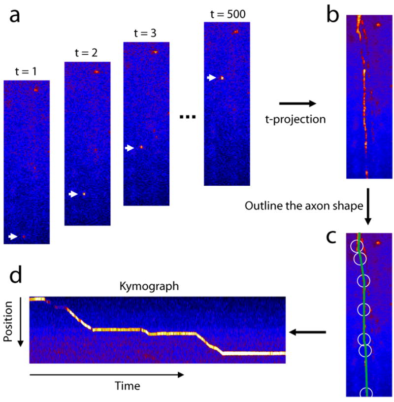
Construction of kymograph image from the time-lapse image series. (a) Index-colored fluorescence images at various time point. (b) Maximum intensity projection of the image series along the time axis. (c) Outline of the axon shape. (d) Kymograph image constructed along the axon line. The corresponding time-lapse movie can be found in the supplementary materials (movie S1).

The kymograph is constructed by defining an ‘observation line’ L along one of these trails in the projection image (Racine et al., 2007; Smal et al., 2010; Stokin et al., 2005; Welzel et al., 2009), e.g. the green line in Figure 1c. Several points on the line are selected out manually (white circles in Figure 1c). Since the line L is not necessarily a straight line across the image, the coordinate d_i along the line L would depends on x and y coordinates on the image. The relation is calculated by linear interpolation of the selected points along line L using pixel-by-pixel equal-distant coordinates (d_i). The total length of L should approximately equal to the trail length in the projection image. The kymograph image I^K(t,d) is assembled from the original data intensity at those coordinates (d_i). Every column t in the kymograph image contains the gray-scale intensity values at locations (d_i) in t^th image. In practice, to increase the signal to noise ratio, the intensity values are obtained by averaging pixel values in the vicinity of d_i along a line perpendicular to L. Figure 1d shows an example of generated kymograph image. The vertical axis is the spatial distance along line L. The width of the kymograph image is identical to the length of the movie sequence. For example, this particular movie sequence consists of 500 frames, therefore the width (in pixels) of the image is also 500. The line trace of a moving particle can be clearly seen. The slope of this line corresponds to the velocity of the particle and the flat segments are time periods when the particle is stationary. Now the problem of identification and localization of moving particles has been transformed to the isolation and extraction of the trace from the kymograph image.

2. Generation of seed points

Curving tracing in an image generally starts from a certain initial point, tracks along the center lines, and terminates at positions where stopping conditions are satisfied (Can et al., 1999; Zhang et al., 2007). We locate the initial seeding points by identifying local intensity maxima within the kymograph. A pixel is considered as local maxima if no other pixel within a distance w is of greater or equal intensity. For this purpose, the kymograph image is first processed by the gray-scale dilation that sets the value of pixel I^K(t,d) to the maximum value within a distance w of coordinates (t,d), as shown in Figure 2b.. Pixel-by-pixel comparison between the dilated image and the original image locates those pixels that have the same value, which are local bright points. Because only the brightest pixels fall onto the axon outline, we further require that candidates for seed point pⁱ to be in the upper 10% percentile of brightness for the entire image (Figure 2c).

Figure 2.

Initial seeding points determination. (a) The kymograph image. (b) Kymograph image after gray-scale dilation. (c) Seed points determined as local maximum overlapped on the kymograph image.

For a high quality kymograph image that contains only one particle trace, a single seeding point is sufficient. However, it is expected that the traces are sometimes segmented due to particles going out of focus or photo-blinking of fluorophores such as quantum dots. In addition, when particle traces cross on the kymograph image, those traces are also separated into segments. The brightness cutoff is set that at least one seed point is detected on every trace segment. Occasionally, some false points not on the trace lines will be recognized as seed points due to uneven fluorescence background along the shape of the axon and bleaching of fluorescence background over time. Those false seed points will be automatically removed during the curve tracing step.

3. Direction estimation by edge detection

After the initial seeding step, a sequence of exploratory searches are initiated at each of the seed point pⁱ for curve tracing in the 2D kymograph image. The process of curve tracing is composed of three steps: (1) determining the line direction vector D⃗ⁱ at a seed point pⁱ; (2) locating the next point pⁱ⁺¹ following the line direction and move to pⁱ⁺¹; and (3) iteratively repeating (1) and (2) until certain termination condition is met. The core tracing algorithm is carried out using an implementation of Steger’s algorithm (Steger, 1998) that is based on detecting the edges of the line perpendicular to the direction of the line and average intensity along the direction the line.

The line direction D⃗ⁱ at point pⁱ is estimated using a combination of edge response and intensity response between a template and the neighborhood of nearby pixels, an algorithm that has been previously reported (Can et al., 1999; Zhang et al., 2007). To be consistent with previous reports, we use similar notations as in Zhang et. al. (Zhang et al., 2007).

For each seed point pⁱ, its surrounding two-dimensional space is discretized into thirty-two equally spaced directions. However, not all thirty-two directions are physically possible. Due to the irreversibility of time, the trace always moves forward along the time axis in a kymograph. Therefore, only sixteen directions are possible, and each direction is indexed by a number (Figure 3a). For any arbitrary direction d⃗, a low-pass differentiator filter is applied to its perpendicular direction in order to detect edge responses. The kernel of the differentiator filter for left and right edge responses are given by:

$$\begin{array}{l}{h}_L[j]=\frac{1}{8}(-\delta [j-2]-2\delta [j-1]+2\delta [j+1]+\delta [j+2])\\ h_R[j]=\frac{1}{8}(\delta [j-2]+2\delta [j-1]-2\delta [j+1]-\delta [j+2])\end{array}$$ (1)

Figure 3.

Line direction estimation by template and intensity responses. (a) Dividing the two-dimensional space to the right of the seed point pⁱ into 16 equally-spaced discrete directions. (b) For each direction d⃗, edge responses are calculated from intensities at various points j. j represents the number of pixels away from the seed point pⁱ along the direction perpendicular to d⃗. (c) The calculated left and right responses vs. j for direction d⃗=12. (d) The plot of template response vs. directions shows a maximum at d⃗=12. (e) The plot of the intensity response vs. direction also shows a maximum at d⃗=12.

Where δ[j] is the discrete unit-impulse function and j represents the number of pixels away from the seed point pⁱ along the direction perpendicular to d⃗ (Figure 3b).

To be consistent with previous reports, we will use (x, y) instead of (t, d) axis notations for kymograph image for this section. Numerically, the calculated (x, y) positions of point j are often not integer numbers. The intensity at point (x, y) is calculated using weighted addition of intensities of four pixels surrounding it.

$$I(x,y)=(1-x_F)(1-y_F)I(x_I,y_I)+x_{F}I(x_I+1,y_I)+y_{F}I(x_I,y_I+1)-x_F{y}_{F}I(x_I+1,y_I+1)$$ (2)

where $\begin{array}{l}x=x_I+x_F\hfill \\ y=y_I+y_F\hfill \end{array}$, and x_I is the integer part of x and x_F is the remaining decimal part. In order to reduce the high-frequency noise, we averaged intensity values over those five points that begins at point j and equally spaced with 1-pixel apart along the orientation of d⃗. The five-point average intensity at j= 0 (i.e. at the location of pⁱ) along the direction d⃗ is denoted as intensity response I(d⃗).

The most probable line direction D⃗ⁱ should give the sharpest edge response among all arbitrary directions d⃗ at point pⁱ (Figure 3c), and any suboptimal line direction d⃗ will lead to flatter edge responses than the optimal one. The left and right edge responses for direction d⃗ at point j are calculated by convoluting intensity vector I[d⃗, j] with the differentiator filter in equation (1) which gives

$$\begin{array}{l}L[\overrightarrow{d},j]=\frac{1}{8}(-I[\overrightarrow{d},j-2]-2I[\overrightarrow{d},j-1]+2I[\overrightarrow{d},j+1]+I[\overrightarrow{d},j+2])\\ R[\overrightarrow{d},j]=\frac{1}{8}(I[\overrightarrow{d},j-2]+2I[\overrightarrow{d},j-1]-2I[\overrightarrow{d},j+1]-I[\overrightarrow{d},j+2])\end{array}$$ (3)

The range of j values was chosen to from −8 to 8 based on the size of the particle in experimental data. Figure 3c illustrates the left and right responses for direction 12 as a function of j. As expected, the left and right responses are of the same absolute value with opposite signs. The maximum values of left and right responses are R_max(d⃗) at j= 2 and L_max(d⃗) at j=−1 along direction d⃗. The overall template response along direction d⃗ is defined as

$$T_{max}(\overrightarrow{d})=max\left\{R_{max}(\overrightarrow{d}),L_{max}(\overrightarrow{d})\right\}$$ (4)

As shown in Figure 3d, the plot of overall template response vs. direction d⃗ shows a maximum at d⃗=12, which is the right line direction. In previous reports (Can et al., 1999; Zhang et al., 2007), only the template response is used for direction estimation, for which the direction with the largest T_max(d⃗) is chosen to be the direction vector D⃗ⁱ for the seed point pⁱ. Here, we also incorporate information in the intensity response I(d⃗) (Figure 3e). In general, the template response T_max(d⃗) is more accurate in finding the right direction vector than the intensity response I(d⃗). However, the kymograph image is much noisier than a real 2D image, which gives rise to noisy template and intensity responses. The template response parameter is susceptible to high frequency noises while the intensity response parameter is more affected by the low frequency intensity variations in the image. We estimate the direction vector by calculating the sum of the template and the intensity responses. Equal weights are chosen for the template and the intensity responses after testing over tens of kymograph images. Therefore, the direction whose combined values of the template response and the intensity response is the maximum among all 16 directions is chosen to be the direction vector D⃗ⁱ for point pⁱ.

$${\overrightarrow{D}}^i=argmax\left\{T_{max}(\overrightarrow{d})+I(\overrightarrow{d})\right\}$$ (5)

4. Curve tracing in kymograph image

After the tracing direction is determined at the seed point pⁱ, the position of next point pⁱ⁺¹ on the curve can be calculated from a pre-defined step size. Since we are interested in the particle position at each time frame that corresponding to a vertical slice on the kymograph image, we trace forward a single pixel in the x axis (time axis). Given the optimal direction vector D⃗ⁱ, the next point pⁱ⁺¹ can be obtained as:

$$\begin{array}{l}{x}^{i+1}=x^i+1\\ y^{i+1}=y^i+tan(arg{\overrightarrow{D}}^i)\end{array}$$ (6)

where arg D⃗ⁱ is the angle of vector D⃗ⁱ.

Even the initial seed point is usually located at the center of the kymograph line, the calculated next point pⁱ⁺¹ does not always fall at the center of the line due to discretized directions and highly pixelated image. As the tracing process proceeds forward, some points can deviate significantly from the kymograph line, particularly at locations when the line makes an abrupt turn (Figure 4a). To move the next point pⁱ⁺¹ closer to the center of the line, we set the algorithm to find the brightest pixel in the vicinity (± 2 pixels) of the calculated yⁱ⁺¹ along the y direction and assign it as the new yⁱ⁺¹. This step will move the next point to the center of the line that is generally the local maximum in y direction. The xⁱ⁺¹ is kept unchanged because each column of data comes from a single time frame. Therefore, the next point pⁱ⁺¹ is moved to the center of the line before calculating the direction vector for the following time point. Figure 4b shows the good agreement between the computed trace and the source kymograph, after each point is adjusted to the center of the line.

Figure 4.

Curve tracing from an initial seed point (shown in green). (a) Direct curve tracing shows significant deviation from the real line, particularly at places where the line changes direction (a′). (b) After adjusting the next point pⁱ⁺¹ to the center of the line after each tracing step, the traced curve accurately follows the real line.

The tracing process is repeated until one of the following termination conditions is met.

1. The next point pⁱ⁺¹ falls within max(j)+1 pixels from the edge of the image.

2. The next point pⁱ⁺¹ falls within the overlap range (± 3 pixels) of a previously detected curve. This condition terminates the tracing at the intersections and avoids repeated tracing.

3. The maximum template response falls below a predefined threshold. This threshold terminates the tracing when the line does not show a clear edge with respect to its local background.

4. The intensity response falls below a predefined sensitivity threshold. This threshold ends the tracing when the brightness of the line is below a certain value.

It should be noted that seed points are not necessarily located at the beginning of the line segment. In order to trace the line to its very beginning, we also apply the curve tracing method to the left side of each seed point for reverse tracing after the forward tracing is terminated. For reverse tracing, the direction estimation, next point calculation and termination conditions are the same as the forward tracing, except for using the negative time (in Eq. 6) and the mirror-image set of discretized direction.

5. Refining spatial positions

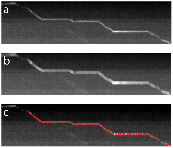
The trajectory data extracted from the curve tracing has a spatial resolution limited by both the accuracy of tracing algorithm and the diffraction of light. During the tracing step, the center of the particle at time t is set to be the brightest pixel in the y direction which sets the spatial resolution to 1 pixel (~0.25 μm) minimum (Figure 5a). The diffraction limit of the light sets the ultimate spatial resolution for any optical microscopy at approximately half wavelength of the light. Most importantly, the “observation line” used to construct the kymograph image is drawn semi-manually, which could deviate from the actual particle center by a few pixels. In order to achieve higher spatial resolution, we refine the position of each trajectory point on the 2D kymograph image by back-projecting them onto their corresponding location in the original three-dimensional movie images. An example is given in Figure 5b that shows a small image area surrounding the circled point shown in Figure 5a in its corresponding time frame. The particle center determined by the curve tracing process (the red dot in Figure 5b) deviates from the real particle center.

Figure 5.

Refining particle positions by back-projection from the kymograph image to the original image series. (a) The trajectory constructed by curve tracing has a spatial resolution about 2 pixels (~0.5μm). (b) Back-projection of a point (dotted circle) in the trajectory to the image series shows deviation from the real center of the particle. (c) Locating the center of the particle by 2D Gaussian fitting. (d) Re-constructed trajectory after fining the position of every point show much higher spatial resolution (~15nm).

Each particle position is refined for better spatial resolution by single particle localization. The central position of an isolated fluorescence emitter can be determined to a high accuracy by fitting their point spread function (PSF) intensity profile with a 2D Gaussian function (Moerner, 2006; Mudrakola et al., 2009; Yildiz et al., 2003). Notably, the precision of this localization is not limited by the spread of its diffraction-limited intensity profile. The localization accuracy of this procedure is only limited by the signal to noise ratio of the image and the total number of photons collected. In practice, accuracies of a few nanometers or less have been achieved. We fit the small image with a symmetric two-dimensional Gaussian function

$$I(x,y)=I_0·exp\left(-\frac{{(x-x_0)}^2+{(y-y_0)}^2}{4{\sigma }^2}\right)$$ (7)

using a simplex algorithm with a least-squares estimator. All four parameters x₀, y₀, σ and I₀ are allowed to vary.

The Gaussian fitted values of x₀and y₀ are added to the estimated values determined in the previous step to obtain better spatial resolution for each point. Figure 5d displays the same trajectory after the position refinement. The localization accuracy of 15nm is achieved, which is estimated from the positional fluctuation in the segment of the trajectory when the particle is stationary.

6. Connecting trace segments by incorporating of global features

In many of cases, multiple particles of varying brightness move in the same axon and their traces can overlap or cross over each other (figure 6a). Our implantation of Steger’s algorithm uses information from several neighboring pixels, but it is unable to work accurately in two situations: (1) curves that fade out and re-appears and (ii) curve following at junctions. Ideally, a curve tracing algorithm should perform as well as human perception. Human vision can detect a line from the whole image (a global view) as well as a cropped one (a local view). Therefore, a good curve tracing algorithm has to incorporate both the local as well as the global features of a line.

Figure 6.

Curve tracing of the kymograph image with poor signal to noise ratio. (a) A representative kymograph image of DiI-labeled vesicle shows many particles of various intensities and their traces overlap and cross over each other. The corresponding time-lapse movie can be found in supplementary materials (movie S2). (b) Curve tracing of the kymograph image shown in figure 6 produces many fragmented traces. (c) Illustration of connecting two trace-fragments by measuring their end-to-end distance and their relative orientation. (d) Selection of optimal connections when two trajectories cross each other. (e) Particle trajectories after connecting trace segments and filling in the gaps.

One of the termination conditions of our tracing algorithm is when the intensity response falls below a predefined sensitivity threshold. If the particle re-appears after a short interval, it will be recognized as a new trajectory (figure 6b). To address this issue, we first trace out the two segments independently and then link them together if certain global conditions indicate that they actually belong to the same trajectory. The possible connections are detected based on relative orientation between two segments and relative distance between their end points. The orientation measure, θ, is defined as

$$\theta ={\theta }_a+{\theta }_b,$$ (8)

where θ_a and θ_b are angles between segments and the connecting line as shown in figure 6c. The relative distance measure is defined as

$$d/(l_a+l_b)$$ (9)

where d is the distance between the end points of two segments and l_a and l_b are their lengths. We accept the connection if it satisfies the condition given by θ< T_θ and d/(l_a+l_b)< T_d where T_θ and T_d are two user defined threshold values. The typical working values of T_θ and T_d are 0.5 and 0.2, respectively, meaning two segmented trajectories apart by 20% of their total lengths and ~28 degrees are likely to be joined as a single trajectory.

In the case of two traces crossing each other, the current tracing algorithm would very likely yield four fragmented trajectories. In this case, there could be multiple possibilities satisfying the connecting condition at the junction. If we follow one trace only, we select one possibility, which is the most likely connection. However, when we consider multiple possible connections simultaneously, we need to find the optimal linkage combination (figure 6d). Therefore, in order to select globally optimal connections, it is necessary to consider all the possible connections simultaneously and choose the optimal one. The optimal connections are chosen by minimizing the summary of all connection measures

$$\sum _i{(\theta +\lambda ·d/(l_a+l_b))}_i$$ (10)

where (θ+λ·d/(l_a+l_b))_i is the measure of i^th linkage and λ is a weight parameter. We empirically choose λ = 3 for our experimental data because d/(l_a+l_b) has a smaller range of value than θ among all putative linkages. After selecting the optimal connections, the gaps of the selected connections are filled by finding the local maximum pixels around the connection line. We extract sufficiently long connected segments, and regard them as particle trajectories as shown in figure 6e. After extracting dynamic trajectories from movies, all subsequent kinetic analysis such as moving velocity, direction, pausing frequency and duration can be computed with ease.

Discussions

In the last decade, extensive studies link impaired axonal transport to a range of human neurodegenerative diseases including Alzheimer’s disease (Stokin et al., 2005), amyotrophic lateral sclerosis (Collard et al., 1995), Parkinson’s disease and frontotemporal dementia (Ittner et al., 2008). In most cases, the average rate of axonal transport is slowed by 20% or less as compared with normal neurons. However, the axonal transport process is intrinsically heterogeneous, with the transport rate of individual cargos varying by an order of magnitude (Cui et al., 2007). In order to draw statistically significant conclusions out of individual cargo transport measurements, one needs to analyze a large number of trajectories. In previous studies, manual tracking of particle trajectories from a time-lapse image series has predominated the analysis. In this procedure, the amount of trajectory data is often limited (tens of trajectories) and the selection criterion is hardly impartial. In contrast, the method presented here is capable of generating >1000 trajectories from a single day experiment.

In this paper, we describe a numerical method for the automatic extraction of particle trajectories during axonal transport. We first transform the problem of particle tracking in a 3D data set as a curve tracing problem in a 2D spatiotemporal kymograph image. Initial seed points are automatically detected as local brightest points. The core tracing algorithm is based on the direction-dependence of the edge and intensity response functions between a template and the neighborhood of nearby pixels. High spatial resolution (~15nm) is achieved by back-projecting the trajectory points located in the kymograph onto the original image data and fitting the particle image with a 2D Gaussian function. After all candidate segments are extracted, an optimization process is then used to select and connect these segments. We have shown experimentally that particle trajectories can be stably extracted by means of this method.

Automated data analysis for axonal transport process would minimize the selection bias and reduce errors and thus can be applied to high throughput image processing. As expected, the performance of the present method still depends on the quality of the data. In images where background fluorescence is high and particle intensities vary by more than 10 times, this method would miss some trajectory segments of the dim particles. In addition, when the particle is very dim and signal to background ratio is low, the 2D Gaussian fitting may not converge, leading to missing points in the high resolution trajectory. Fully automated axon line detection is still in progress.

Supplementary Material

Supp 01. Movie S1.

Retrograde transport of Qdot-NGF in DRG neurons

Supp 02. Movie S2.

Anterograde transport of DiI-labeled vesicles in DRG neurons.

References

- Bronfman FC, Tcherpakov M, Jovin TM, Fainzilber M. Ligand-induced internalization of the p75 neurotrophin receptor: a slow route to the signaling endosome. J Neurosci. 2003;23:3209–3220. doi: 10.1523/JNEUROSCI.23-08-03209.2003. [DOI] [PMC free article] [PubMed] [Google Scholar]
- Can A, Shen H, Turner JN, Tanenbaum HL, Roysam B. Rapid automated tracing and feature extraction from retinal fundus images using direct exploratory algorithms. IEEE Trans Inf Technol Biomed. 1999;3:125–138. doi: 10.1109/4233.767088. [DOI] [PubMed] [Google Scholar]
- Carter BC, Shubeita GT, Gross SP. Tracking single particles: a user-friendly quantitative evaluation. Phys Biol. 2005;2:60–72. doi: 10.1088/1478-3967/2/1/008. [DOI] [PubMed] [Google Scholar]
- Cheezum MK, Walker WF, Guilford WH. Quantitative comparison of algorithms for tracking single fluorescent particles. Biophys J. 2001;81:2378–2388. doi: 10.1016/S0006-3495(01)75884-5. [DOI] [PMC free article] [PubMed] [Google Scholar]
- Chetverikov D, Verestoy J. Feature point tracking for incomplete trajectories. Computing. 1999;62:321–338. [Google Scholar]
- Collard JF, Cote F, Julien JP. Defective axonal transport in a transgenic mouse model of amyotrophic lateral sclerosis. Nature. 1995;375:61–64. doi: 10.1038/375061a0. [DOI] [PubMed] [Google Scholar]
- Crocker JC, Grier DG. Methods of digital video microscopy for colloidal studies. Journal of Colloid and Interface Science. 1996;179:298–310. [Google Scholar]
- Cui B, Wu C, Chen L, Ramirez A, Bearer EL, Li WP, Mobley WC, Chu S. One at a time, live tracking of NGF axonal transport using quantum dots. Proc Natl Acad Sci U S A. 2007;104:13666–13671. doi: 10.1073/pnas.0706192104. [DOI] [PMC free article] [PubMed] [Google Scholar]
- Falnikar A, Baas PW. Critical roles for microtubules in axonal development and disease. Results Probl Cell Differ. 2009;48:47–64. doi: 10.1007/400_2009_2. [DOI] [PubMed] [Google Scholar]
- Holzbaur EL. Motor neurons rely on motor proteins. Trends Cell Biol. 2004;14:233–240. doi: 10.1016/j.tcb.2004.03.009. [DOI] [PubMed] [Google Scholar]
- Ittner LM, Fath T, Ke YD, Bi M, van Eersel J, Li KM, Gunning P, Gotz J. Parkinsonism and impaired axonal transport in a mouse model of frontotemporal dementia. Proc Natl Acad Sci U S A. 2008;105:15997–16002. doi: 10.1073/pnas.0808084105. [DOI] [PMC free article] [PubMed] [Google Scholar]
- Kannan B, Har JY, Liu P, Maruyama I, Ding JL, Wohland T. Electron multiplying charge-coupled device camera based fluorescence correlation spectroscopy. Anal Chem. 2006;78:3444–3451. doi: 10.1021/ac0600959. [DOI] [PubMed] [Google Scholar]
- Li H, Li SH, Yu ZX, Shelbourne P, Li XJ. Huntingtin aggregate-associated axonal degeneration is an early pathological event in Huntington’s disease mice. J Neurosci. 2001;21:8473–8481. doi: 10.1523/JNEUROSCI.21-21-08473.2001. [DOI] [PMC free article] [PubMed] [Google Scholar]
- Lochner JE, Kingma M, Kuhn S, Meliza CD, Cutler B, Scalettar BA. Real-time imaging of the axonal transport of granules containing a tissue plasminogen activator/green fluorescent protein hybrid. Mol Biol Cell. 1998;9:2463–2476. doi: 10.1091/mbc.9.9.2463. [DOI] [PMC free article] [PubMed] [Google Scholar]
- Miller KE, Sheetz MP. Axonal mitochondrial transport and potential are correlated. J Cell Sci. 2004;117:2791–2804. doi: 10.1242/jcs.01130. [DOI] [PubMed] [Google Scholar]
- Moerner WE. Single-molecule mountains yield nanoscale cell images. Nat Methods. 2006;3:781–782. doi: 10.1038/nmeth1006-781. [DOI] [PMC free article] [PubMed] [Google Scholar]
- Mudrakola HV, Zhang K, Cui B. Optically resolving individual microtubules in live axons. Structure. 2009;17:1433–1441. doi: 10.1016/j.str.2009.09.008. [DOI] [PMC free article] [PubMed] [Google Scholar]
- Pelkmans L, Kartenbeck J, Helenius A. Caveolar endocytosis of simian virus 40 reveals a new two-step vesicular-transport pathway to the ER. Nat Cell Biol. 2001;3:473–483. doi: 10.1038/35074539. [DOI] [PubMed] [Google Scholar]
- Pelzl C, Arcizet D, Piontek G, Schlegel J, Heinrich D. Axonal guidance by surface microstructuring for intracellular transport investigations. Chemphyschem. 2009;10:2884–2890. doi: 10.1002/cphc.200900555. [DOI] [PubMed] [Google Scholar]
- Racine V, Sachse M, Salamero J, Fraisier V, Trubuil A, Sibarita JB. Visualization and quantification of vesicle trafficking on a three-dimensional cytoskeleton network in living cells. Journal of Microscopy-Oxford. 2007;225:214–228. doi: 10.1111/j.1365-2818.2007.01723.x. [DOI] [PubMed] [Google Scholar]
- Roy S, Zhang B, Lee VM, Trojanowski JQ. Axonal transport defects: a common theme in neurodegenerative diseases. Acta Neuropathol. 2005;109:5–13. doi: 10.1007/s00401-004-0952-x. [DOI] [PubMed] [Google Scholar]
- Salehi A, Delcroix JD, Belichenko PV, Zhan K, Wu C, Valletta JS, Takimoto-Kimura R, Kleschevnikov AM, Sambamurti K, Chung PP, Xia W, Villar A, Campbell WA, Kulnane LS, Nixon RA, Lamb BT, Epstein CJ, Stokin GB, Goldstein LS, Mobley WC. Increased App expression in a mouse model of Down’s syndrome disrupts NGF transport and causes cholinergic neuron degeneration. Neuron. 2006;51:29–42. doi: 10.1016/j.neuron.2006.05.022. [DOI] [PubMed] [Google Scholar]
- Sbalzarini IF, Koumoutsakos P. Feature point tracking and trajectory analysis for video imaging in cell biology. J Struct Biol. 2005;151:182–195. doi: 10.1016/j.jsb.2005.06.002. [DOI] [PubMed] [Google Scholar]
- Smal I, Grigoriev I, Akhmanova A, Niessen W, Meijering E. Microtubule Dynamics Analysis Using Kymographs And Variable-Rate Particle Filters. IEEE Trans Image Process. 2010 doi: 10.1109/TIP.2010.2045031. [DOI] [PubMed] [Google Scholar]
- Steger C. An unbiased detector of curvilinear structures. Ieee Transactions on Pattern Analysis and Machine Intelligence. 1998;20:113–125. [Google Scholar]
- Stokin GB, Lillo C, Falzone TL, Brusch RG, Rockenstein E, Mount SL, Raman R, Davies P, Masliah E, Williams DS, Goldstein LS. Axonopathy and transport deficits early in the pathogenesis of Alzheimer’s disease. Science. 2005;307:1282–1288. doi: 10.1126/science.1105681. [DOI] [PubMed] [Google Scholar]
- Taylor AM, Rhee SW, Jeon NL. Microfluidic chambers for cell migration and neuroscience research. Methods Mol Biol. 2006;321:167–177. doi: 10.1385/1-59259-997-4:167. [DOI] [PubMed] [Google Scholar]
- Vale RD. The molecular motor toolbox for intracellular transport. Cell. 2003;112:467–480. doi: 10.1016/s0092-8674(03)00111-9. [DOI] [PubMed] [Google Scholar]
- Welzel O, Boening D, Stroebel A, Reulbach U, Klingauf J, Kornhuber J, Groemer TW. Determination of axonal transport velocities via image cross- and autocorrelation. Eur Biophys J. 2009;38:883–889. doi: 10.1007/s00249-009-0458-5. [DOI] [PubMed] [Google Scholar]
- Wu C, Ramirez A, Cui B, Ding J, Delcroix JD, Valletta JS, Liu JJ, Yang Y, Chu S, Mobley WC. A functional dynein-microtubule network is required for NGF signaling through the Rap1/MAPK pathway. Traffic. 2007;8:1503–1520. doi: 10.1111/j.1600-0854.2007.00636.x. [DOI] [PubMed] [Google Scholar]
- Yildiz A, Forkey JN, McKinney SA, Ha T, Goldman YE, Selvin PR. Myosin V walks hand-over-hand: single fluorophore imaging with 1.5-nm localization. Science. 2003;300:2061–2065. doi: 10.1126/science.1084398. [DOI] [PubMed] [Google Scholar]
- Zhang K, Osakada Y, Vrljic M, Chen L, Mudrakola HV, Cui B. Single molecule imaging of NGF axonal transport in microfluidic devices. Lab on a Chip. 2010 doi: 10.1039/c003385e. In press. [DOI] [PMC free article] [PubMed] [Google Scholar]
- Zhang Y, Zhou X, Degterev A, Lipinski M, Adjeroh D, Yuan J, Wong ST. A novel tracing algorithm for high throughput imaging Screening of neuron-based assays. J Neurosci Methods. 2007;160:149–162. doi: 10.1016/j.jneumeth.2006.07.028. [DOI] [PubMed] [Google Scholar]
Associated Data
This section collects any data citations, data availability statements, or supplementary materials included in this article.
Supplementary Materials