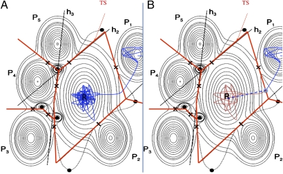
Fig. 2.

Schematic contour plot of an energy surface showing an initial state minimum, R, and five possible final state minima, P₁–P₅. Maxima are denoted with filled circles, and saddle points are denoted by ×. In the harmonic approximation (the case illustrated here), the dividing surfaces are hyperplanar segments containing a first-order saddle point and oriented with the normal pointing along the unstable mode. (A) A reactive classical trajectory requires impossibly long simulations of vibrations in the initial state until a transition is observed (blue line). (B) In the WKE procedure, a short trajectory containing the essential information is generated in the following way. A statistical estimate is made of the time needed to reach a point (denoted by an open blue circle) in the transition state, a short trajectory from that point forward in time is generated to determine the final state (blue line), and a short trajectory backward in time is generated to verify that it originated in the initial state (red line); otherwise, a new trajectory is generated. The configuration space is partitioned into subspaces by dividing surfaces (straight red lines), and long time-scale simulation using the adaptive kinetic Monte Carlo (AKMC) method tracks the advance of the system from one subspace to another.