Figure 3.

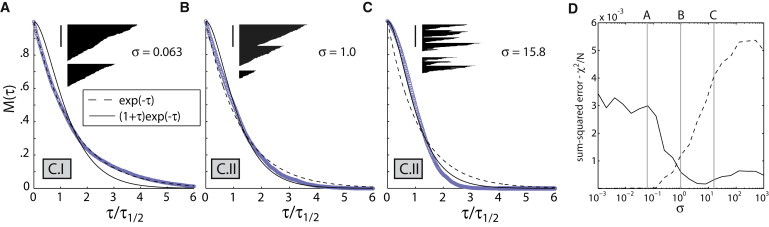
Severing generates nonexponential polymer mass decay curves. (A–C) Kymographs of single filaments and corresponding polymer mass decay curves for severing-based turnover (Model C), shown for parameters corresponding to regime C.I (A) and regime C.II (B and C). The values of σ = k_sv²₊/k²_cv₋ for each plot are shown. Two example filament kymographs are shown for each set of parameters, with time on the x axis and subunits on the y axis. Vertical bar = 100 subunits; barbed ends point upwards. For each plot, polymer mass decay curves (circles) represent ensemble average of simulated single-filament trajectories. For each plot, kymographs and decay curves share the same time axis, which is scaled such that one unit represents the time required for the polymer mass to decay to half its initial value (τ_1/2). Thin smooth lines represent best fits of simulated polymer mass decay curves to a single exponential (dashed) and an inflected exponential (solid). (D) Curve showing sum-squared errors (χ²/N) for best fits to a simple exponential (dashed) and an inflected exponential (solid) for different values of σ. Values of σ used for simulations in panels A–C are shown with vertical bars. In all simulations, k_s was varied while all other parameters were kept constant at v_– = 10, 〈L〉 = v₊/k_c = 100.