Figure 4.

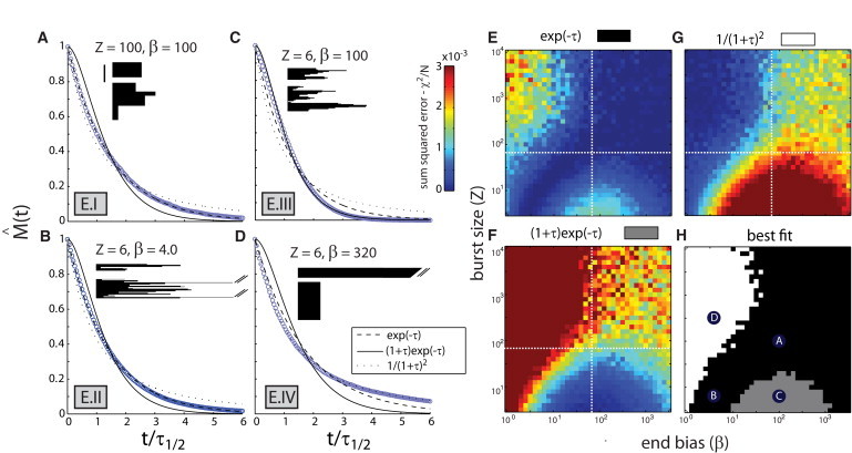
Bursting disassembly can generate exponential polymer mass decay curves. (A–D) Kymographs and polymer mass decay curves for bursting filament turnover (Model E), shown for parameters corresponding to Regimes E.I (A), E.II (B), E.III (C), and E.IV (D). The values of burst size Z and end bias β used for each plot are shown. Two example filament kymographs are shown for each set of parameters, with time on the x axis and subunits on the y axis. Vertical bar = 100 subunits. Polymer mass decay curves (blue) represent ensemble average of simulated single-filament trajectories. For each plot, kymographs and decay curves share the same time-axis, which is scaled such that one unit represents the time required for the polymer mass to decay to half its initial value. Smooth curves (black) represent best fits to simulated polymer mass decay curves. (E–G) Two-dimensional surface plots showing sum-squared errors (χ²/N) for best fits of different analytical curves to simulated curves as a function of β and Z. White-dotted lines give the value of 〈L〉 used in simulations. (H) Two-dimensional plot showing the regions in (β, Z) space where a given curve's best-fit has the smallest χ²/N value [exp(– τ), black; (1 + τ) exp(– τ), gray; 1/(1 + τ)², white]. Labeled circles denote the parameter values used for simulations in panels A–D. Other values: 〈L〉 = v₊/k_c = 70.