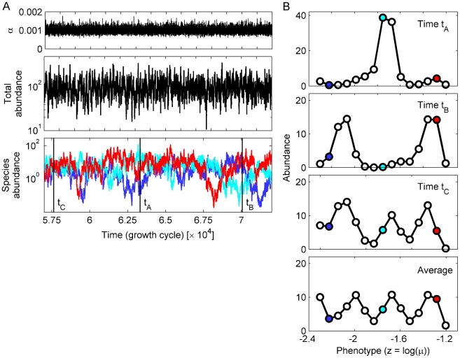
Figure 3. Environmental noise leads to clusters of abundant species in phenotype space.

(A) Time-trace of the system from Figure 2 in the presence of noise in the dispersal dilution factor α. From top to bottom, the panels show: time-traces of α, the total per-patch abundance, and the per-patch abundances of the three representative species from Figure 2A. The dilution rate is drawn independently every cycle from a log-normal distribution with a coefficient of variation of σ_α/<α> = 0.15. The total and individual abundances vary over several orders of magnitudes, with different species taking turns being the most abundant. (B) Examples of the species abundances profile in phenotype space at specific times (t_A, t_B, t_C; indicated by vertical black lines in panel B), and the time-averaged profile. The species are arranged by increasing growth rate (the x-coordinates are z_k = log(μ_k)). The top three panels show cases of one, two, and three dominant peaks, examples of the typical peak-and-valley pattern induced by the environmental noise (see also Supplementary Figures S3 and S4). The number, position, and height of the peaks vary across time, but the uneven distribution remains when averaging over 50,000 time steps (bottom panel). Colored dots indicate the three representative species from panel A.