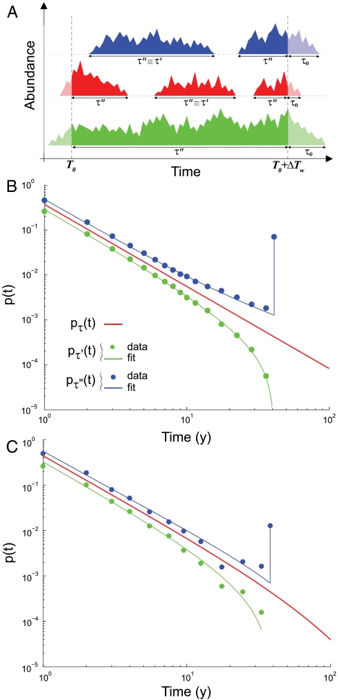
Fig. 2.

Empirical persistence-time distributions. (A) A schematic representation of the variables that can be measured from empirical data over a time window ΔT_w: τ^′, persistence times that start and end inside the observational window, and τ^′′ , which comprises τ^′ and all the portions of persistence times seen inside the time window that start or/and end outside. Times to local extinction τ_e are also presented. (B) Breeding birds and (C) herbaceous plants probability density function p(t) of τ^′ (green), τ^′′ (blue), and persistence time τ (red). Filled circles and solid lines show observational distributions and fits, respectively. The best fit is achieved with p_τ(t) ∝ t^-α with α = 1.83 ± 0.02 and α = 1.78 ± 0.08 for breeding birds and herbaceous plants, respectively. Note that previous estimates (6) for B are revisited here in the light of the tools developed and of a longer dataset. The spatial scale of analysis is A = 10,000 km² and ΔT_w = 41 y for B and A = 1 m² and ΔT_w = 38 y for C. The finiteness of the time window imposes a cutoff to p_τ^′(t) and an atom of probability in t = ΔT_w to p_τ^′′(t), which corresponds to the fraction of species that are always present during the observational time. p_τ(t) and p_τ^′(t) have been shifted in the log–log plot for clarity.