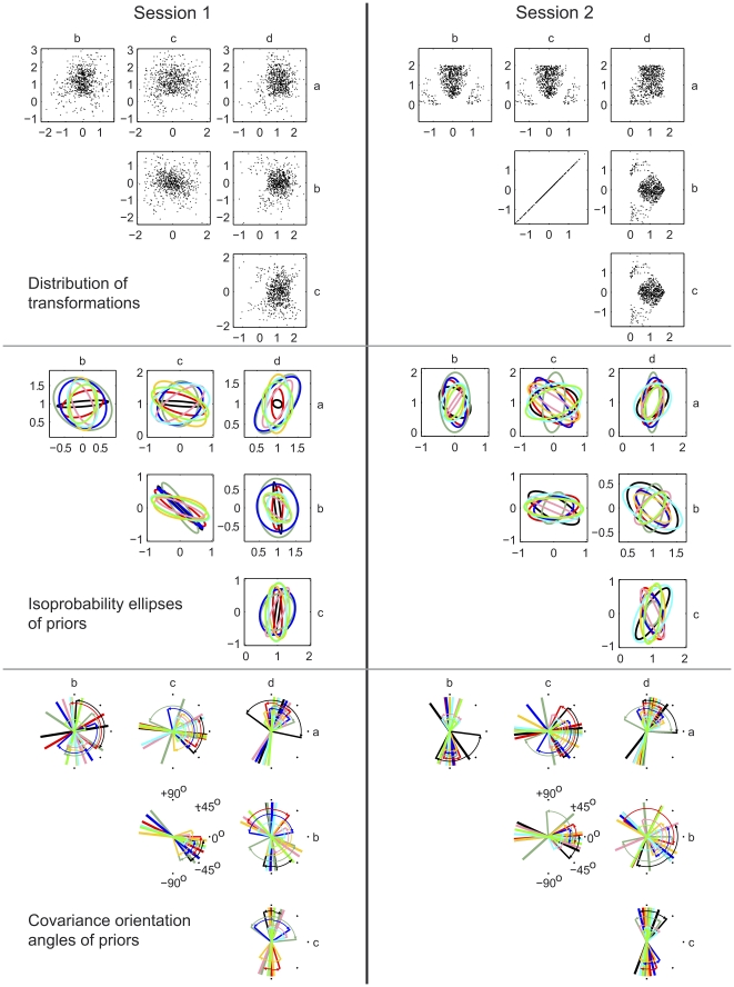
Figure 5. Distributions of transformations and prior distributions in Sessions 1 and 2.

Left column: Session 1. Right column: Session 2. Top row: the distributions of transformations in the two sessions. In each case 700 of the experimental transformations are plotted in the six projections of the 4-D space of linear transformations used in Figure 4. Middle row: the priors fit to the data of the 8 subjects, plotted in the style used for the priors in Figure 4. Each covariance matrix has been scaled so that its largest eigenvalue is unity, in order that all priors can be displayed together without any being too small to see. Bottom row: confidence limits on covariance orientation angles, shown for each pairing of the four elements of the transformation matrix , , , . These confidence limits were obtained by bootstrapping, as explained in Methods. For each subject, thick lines show the mean angle across the 1000 or more resampled fits. Thin lines, connected to the mean line by curved arrows, give the 95% confidence limits. Only the range to is labelled, because the data is axial and therefore only exists in a 180 range.