Abstract
Background and Aims
Epidemiological simulation models coupling plant growth with the dispersal and disease dynamics of an airborne plant pathogen were devised for a better understanding of host–pathogen dynamic interactions and of the capacity of grapevine development to modify the progress of powdery mildew epidemics.
Methods
The first model is a complex discrete mechanistic model (M-model) that explicitly incorporates the dynamics of host growth and the development and dispersion of the pathogen at the vine stock scale. The second model is a simpler ordinary differential equations (ODEs) compartmental SEIRT model (C-model) handling host growth (foliar surface) and the ontogenic resistance of the leaves. With the M-model various levels of vine development are simulated under three contrasting climatic scenarios and the relationship between host and disease variables are examined at key periods in the epidemic process. The ability of the C-model to retrieve the main dynamics of the disease for a range of vine growth given by the M-model is investigated.
Key Results
The M-model strengthens experimental results observed regarding the effect of the rate of leaf emergence and of the number of leaves at flowering on the severity of the disease. However, it also underlines strong variations of the dynamics of disease depending on the vigour and indirectly on the climatic scenarios. The C-model could be calibrated by using the M-model provided that different parameters before and after shoot topping and for various vigour levels and inoculation time are used. Biologically relevant estimations of the parameters that could be used for its extension to the vineyard scale are obtained.
Conclusions
The M-model is able to generate a wide range of growth scenarios with a strong impact on disease evolution. The C-model is a promising tool to be used at a larger scale.
Keywords: Host–pathogen models, mechanistic model, SEIRT model, host growth, powdery mildew, grapevine
INTRODUCTION
The grape–powdery mildew pathosystem is characterized by a polycyclic pathogen capable of explosive multiplication and a host population with a high degree of spatial structure at the field level and a complex architecture at the individual plant level exhibiting rapid changes over time. As well as environmental differences, the high degree of human interference during vine development and the wide diversity of cropping systems enhance variability from one crop to another. Furthermore, because of the close relationship between powdery mildew and its host (Doster and Schnathorst, 1985; Gadoury et al., 2003) and of the spatial location of primary infections on the vine stock, we hypothesize that the dynamic changes in crop structure should be considered as key factors for explaining variability in the severity of epidemic behaviour. Indeed, by modifying the movement of inoculum, or by altering the susceptibility of the leaf population, natural and management-induced changes in crop growth and crop architecture may significantly affect the course of the epidemics (Calonnec et al., 2009).
For a better understanding of these host–pathogen dynamic interactions and of the capacity of host development to modify the disease progress, epidemiological simulation models have been developed coupling plant growth with the dispersal and disease dynamics of the airborne plant pathogen, Erysiphe necator. The first model developed (Calonnec et al., 2008) is a complex discrete deterministic model that explicitly incorporates the dynamics of host growth and the development and dispersion of the pathogen. In this model, input variables are environmental (daily average temperature, maximum wind speed and average wind direction) or related to the pathogen (location and onset of primary infection). Input parameters characterize the crop system (number of buds, distance between buds, date and height of shoot topping, and vigour), the conditions of growth for the vine and the pathogen (infection, sporulation, dependence on temperature and leaf age) and the dispersion. Outputs describe, at each time step, the number, age and pattern of the healthy and infected organs, infected and infectious leaf area and the aerial density of the spores released. The development of the spatial arrangement of host organs within the vine stock is captured with a 3-D architectural model. It allows simulation of the spatio-temporal dynamics of host growth and epidemic development beginning from a range of climatic conditions, production systems (number of shoots and distance between buds) and initial conditions for the density and location of the pathogen. In particular, this model takes into account shoot topping, which has the effect of enhancing the development of secondary shoots, and then the emergence of new susceptible leaves during the epidemic process.
The second model is a SEIRT model, an extension of the HLSR (Healthy, Latent, Sporulating, Removed) compartmental model (Segarra et al., 2001), which falls in the class of SEIR (Susceptible, Exposed, Infectious, Removed) models in epidemiology. These time-continuous models are systems of ordinary differential equations. In the case of powdery mildew of grapevine, as the time scales of the host growth and of the evolution of the disease are of the same order of magnitude, the host growth cannot be neglected. Our SEIRT model takes also into account the ontogenic resistance of the leaves. It does not take into account explicitly climate or production systems such as shoot topping. The model also uses composite epidemiological parameters assumed to be constant for the sake of simplification, whereas they may depend on the environment. As an example, the rate of disease transmission could depend on the dispersion process but it could also depend on the host density and susceptibility, and therefore on the date of disease initiation. The idea is to develop a model easier to handle than the discrete model from the perspective of up-scaling the study at a vineyard scale with crop heterogeneities for growth and susceptibility. We had already developed a reaction–diffusion model at the vineyard scale (Burie et al., 2007) where the evolution of the disease is locally described by a SEIR model coupled with a set of equations for the dispersal of spores. This model took into account host growth and a true mass action contact term but not the ontogenetic resistance and crop management. Before using this type of model at the plot scale, we needed to investigate the ability of a SEIRT non-spatial model to retrieve variations of vine growth and disease dynamics at the vinestock scale.
In this article, we first examine the relationship between host and disease variables at key periods in the epidemic process for various conditions of vine vigour and climatic conditions by using the discrete model. Then, we fit the SEIRT model to the output of the discrete model in order to obtain parameters corresponding to realistic conditions of disease development and vinestock growth. The relationships between these parameters depending on the environmental conditions (vine growth and climatic scenario) and disease initiation are discussed.
MATERIALS AND METHODS
A discrete mechanistic simulation model
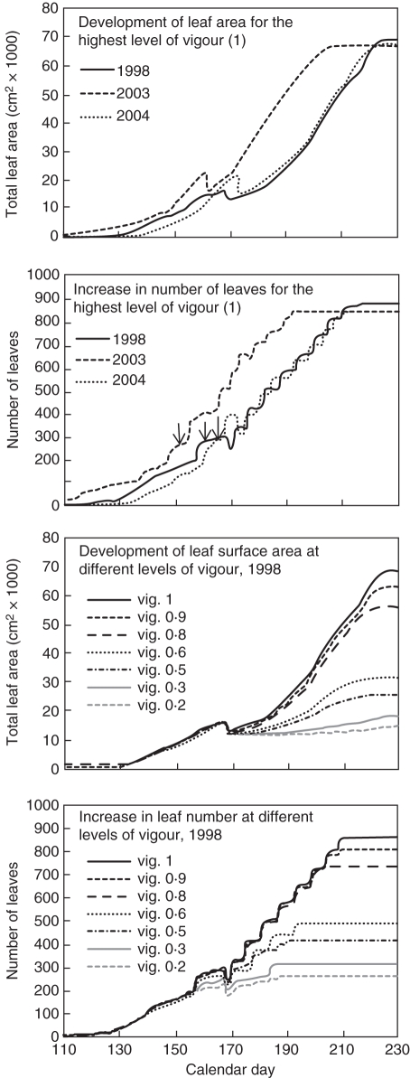
In order to identify favourable or unfavourable effects of crop growth on the dynamics of epidemics, we simulate with the mechanistic model (Calonnec et al., 2008) epidemics for vine growth parameters that reflect various conditions of vine vigour and three climatic scenarios. (a) Seven levels of vine vigour; these levels result in an increased number and development of secondary shoots (Fig. 1), mainly after shoot topping. (b) Three contrasting seasons: 2003 characterized by an early bud break (day 104) and an early flowering (day 152); 1998 a late bud break (day 114) and late flowering (day 159); and 2004, later bud break (day 118) and later flowering (day 163) with an increased development between flowering and shoot topping compared with 1998 (Fig. 1). Day of bud break and day of flowering are achieved when the accumulated sum of the mean daily temperature above 10 °C reaches 90 and 380, respectively, starting from day 1 (1 January). Shoot topping was simulated 10 d after flowering. The vine is simulated with eight buds and contamination is set on the first expended leaf on shoot 4. All the other parameters used are described in Calonnec et al. (2008).
Fig. 1.
Comparison of the total leaf area and of the leaf numbers per vine for various climatic conditions (1998, 2003 and 2004) and vine vigour (0·2–1). Arrows indicate flowering.
Variables used to characterize the host growth were: (a) the rate of leaf emergence (RLE) between the first sporulating event and flowering; (b) the number of leaves at flowering time (Nflo); (c) the leaf surface at flowering (Sflo); and (d) the leaf surface at shoot topping (Sst). The variables used to characterize disease were (a) the rate of diseased leaves emergence (RDLE); (b) the number of infected leaves at flowering (Niflo); (c) the disease leaf surface at shoot topping (SDst); and (d) the disease leaf surface at the end of the epidemic (SD240). Flowering and shoot topping are key periods in the epidemic process: (a) the amount of disease at flowering is correlated to the damage on bunches of grapes on a susceptible cultivar such as as Cabernet-Sauvignon (Peyrard et al., 2005; Calonnec et al., 2006) and (b) at shoot topping the enhanced development of secondary shoots results in an increased amount of susceptible tissue. It is therefore important to retrieve with the model the fact that variation of host growth early in the season has an impact on the disease level.
Data analyses
A principal component analysis and a PLS-path modelling analysis (Tenenhaus et al., 2005) were performed to explore preliminarily the relationships between host development, disease variables and climatic scenarios, and to quantify the weight of each component. The PLS-path model is described by four unobservable or latent variables (LVs) (years, vine growth, crop management and disease). Each LV is constructed by a set of observable or manifest variables (MVs). The variable years are described by three MVs: the inverse of the sum of temperatures >10 °C between bud break and flowering (1/T Bud-Flo), or between flowering and d 240 (1/T Flo-240) and the date of bud break (Dbud); whereas vine growth and disease are described by the same variables as those used for the component analysis, Sflo, Nflo, RLE and Niflo, and RDLE, SDst and SD240, respectively. Finally, the crop management is described by the seven levels of vigour. The standardized latent variables are estimated as linear combinations of their centred MVs. The PLS-path model is described by the measurement model relating the different MVs to their own LVs and the structural model relating the endogenous LV ‘disease’ to the other LVs: ‘vine growth’ and ‘years’. The entire model is important for determining the impact on the main target variable, the disease. The principal component analysis is performed by using the software R (Version 2.1.1, copyright 2005, library ADE4) and the PLS-path modelling by using XSstat-Pro, module PLS-PM (Version 2010.2.02, copyright Addinsoft 1995–2009).
A continuous simulation model
We use a model similar to the HLSR model in Segarra et al. (2001) with the following variants: (a) our model takes into account the host growth and the ontogenetic resistance of the leaves and (b) the contact term is frequency dependent, also called true mass action (de Jong et al., 1995; Ferrandino, 2008) rather than mass action. The unit considered for the state variables is the foliar surface (cm2). The total surface with respect to time is denoted by N(t) and is sub-divided into five compartments: susceptible, S; exposed (latent), E; infectious (sporulating), I; removed since post-infectious, R; and immune due to ontogenic resistance, T, so that N = S + E + I + R + T. The total healthy surface is (S + T). The model equations read:
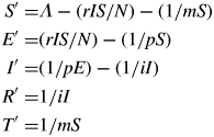 |
The model has five parameters: the disease transmission rate r [(infected surface)·(infectious surface)−1·d−1], the mean period of susceptibility of the foliar surface to the disease m (d) before ontogenic resistance, the mean latent period p (d) and the infectious period i (d).
We assume that the disease has no consequences on the host growth as we have no reference or experimental evidence to confirm or to refute such an assumption: the rate S' of change of the healthy foliar surface is equal to the rate of increase of the new foliar surface given by some function Λ that will be determined thereafter minus the rate at which the foliar surface becomes infected (latent) according to the true mass action contact term r I S/N and minus the rate at which it becomes resistant due to ageing. The time interval for which a unit of healthy surface remains susceptible is given by an exponential law of parameter m.
The rates of changes of E, I, R and T are defined similarly. As in Segara et al. (2001), we neglect the variation of the surface of the colony by assuming it reaches its maximum size as soon as the foliar surface is contaminated. A unit of susceptible surface may become resistant due to ageing and enter compartment T, or it will first become latent (compartment E), then sporulating (I) and finally post-sporulating (R). In particular the period of time a unit of foliar surface stays in compartment E and I also follows an exponential law of parameters p and i, respectively.
We conclude the model presentation by determining Λ explicitly. We assume that the total foliar surface N follows a logistic law of parameters α and K, which is the result of the production and growth of leaves, hence Λ = N' = αN (1 – N/K). N is the well-known solution of the logistic equation with N(0) = N0, this yields:
Parameter assumptions
According to the literature (Analytis, 1980; Gessler and Blaise, 1992), the latent period p depends on the temperature and varies between 7 and 15 d during the season. In the mechanistic model, p is a function of temperature, but in the SEIRT model, for the sake of simplification, we set p to be a constant equal to 10 d (mean and mode value of the corresponding varying parameter of the mechanistic model). Also the infectious period i may vary between 5 and 35 d according to the literature (Chellemi and Marois, 1991), but it is very difficult to assess because of the overlap between primary and secondary inoculation and of colony growth. We can, however, reasonably derive from field experiments the infectious period i to be about 10 d. This is the case for artificial inoculation (primary inoculation identified) and when measuring the duration of the first sporulating event with spore samplers. For both models i is set to 10 d. The susceptibility period before ontogenic resistance (resistance with tissue ageing) decreases following an exponential law in the mechanistic model for each leaf (Calonnec et al., 2008); in the SEIRT model, m is an analogous parameter for the whole vinestock and it is set to 10 d.
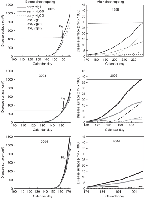
The other parameters of the model, α, K and r, are fitted by non-linear least square regression. These last parameters were estimated by fitting outputs of the mechanistic model based on simulations for three years (1998, 2003 and 2004), three vigour levels (0·2, 0·6 and 1) and two inoculation dates corresponding to the phenological stages of the first and fourth expanded leaves (Fig. 2). In a first step, parameters α and K of the logistic law were fitted to the daily foliar surface area (N) given by the mechanistic model. Then in a second step the rate of disease transmission r was fitted to the daily diseased surface (D = I + R); D is naturally smoothed since it is a time-integrated quantity.
Fig. 2.
Simulation of the diseased surface area generated by the deterministic model as a function of the vigour (0·2, 0·6 and 1), climatic conditions (1998, 2003 and 2004) and the phenological stage at inoculation (early = inoculation at the first expanded leaf stage, late = inoculation at the fourth expanded leaf stage). The disease surface area at flowering (Flo) is indicated in the left-hand graphs and the maximum value for vigour = 1 is indicated in the right-hand graphs.
The simulation starts at bud break t0. The model is used three times successively over the period of simulation with different initial conditions. (1) From bud break t0 to initial contamination day tinf: the initial foliar surface N0 at bud break is taken from the output of the mechanistic model, we thus set S(t0) = N0, T(t0) = 0 and E(t0) = I(t0) = R(t0) = 0. (2) From initial contamination day tinf to shoot topping day tst: we pause the simulation at day tinf and introduce the disease by setting E(tinf) = E0 and replacing the value of S(tinf) with S(tinf) – E0, where E0 is given by the mechanistic model output. More precisely E0 is taken to be equal to the final size of the first colony once it starts sporulating. This size may vary depending on the temperature. For the other compartments, we set I(tinf) = R(tinf) = 0, and the value of T(tinf) does not change from (1). Note that at tinf part of the healthy tissue is not susceptible anymore, i.e. T(tinf) >0. (3) From shoot topping tst to the end of the growth period tend: as it is not possible to know from the actual output of the mechanistic model the quantities subtracted in each compartment at shoot topping, the following assumption is made: the proportion in each compartment immediately before and after shoot topping is conserved.
Hence two sets of parameters α, K and r are computed to take into account the different dynamics before and after shoot topping.
Computations were done with scilab software [scilab-4.1.1, copyright 1989–2007, Consortium Scilab (INRIA, ENPC)]. The model equations are solved using the function ode. Parameter estimation is performed with a quasi-Newton algorithm (function leastsq). The fit quality J is given by the sum of squared residuals divided by the number of daily outputs minus the number of estimated parameters.
RESULTS
A discrete mechanistic simulation model
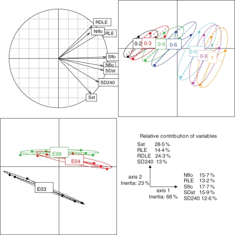
Based on the simulations, the vigour was effectively characterized by a higher number and surface of leaves at flowering (Nflo and Sflo) and a higher rate of leaf emergence (RLE) (Fig. 3). These variables are well represented by the first principal component axis. The RLE was correlated with the number of infected leaves at flowering (Niflo) (correlation coefficient = 0·718) and the rate of diseased leaf emergence (RDLE) (correlation coefficient = 0·954). An increased level of vigour has, as a consequence, an increased level of disease surface area at shoot topping (SDst). Axis 2, mainly explained by the leaf surface at shoot topping (Sst) and the RDLE, allowed discrimination between the climatic scenarios especially for the highest levels of vigour. For example, 2003 shows a higher level of disease late in the season (SD240) than 1998 and 2004. This means that, depending on the climatic conditions, the disease dynamics can be modified.
Fig. 3.
Correlation graph between variables according to a principal component analysis based on: the rate of leaf emergence (RLE), the number of leaves at flowering (Nflo), the rate of diseased leaf emergence (RDLE), the number of infected leaves at flowering (Niflo), and the disease leaf surface at shoot topping (SDst) and at the end of the epidemic (SD240). Individuals from the same vigour level (0·2–1) or from the same year (E98, E03 and E04) are joined by the same colour on the graph of principals.
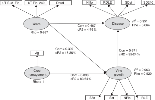
The PLS-path scheme indicates that disease and vine growth are well described by their two latent variables vine growth and years, and years and crop management, respectively (Fig. 4; R2 >0·95 and Dillon–Goldstein's ρ >0·7). The disease is well described by each of the chosen manifest variables (cross-loadings >0·7), with the highest correlation for SDst. Vine growth is the main contributor of disease variation (relative contribution = 95·2 %) and vigour is the main contributor to the variation of vine growth (relative contribution = 83·6 %) compared with years (relative contribution = 16·4 %). The disease is well correlated to vine growth (correlation 0·97 with a path coefficient of 1·008, relative contribution = 95·2 %) through the indirect effects of vigour and years. The direct effect of years, through the temperature, on the disease is weak (relative contribution = 4·7 %). This means that in our simulations the main variability in the disease is due to the strong variations of vine growth mainly because of vine vigour. Among the vine growth variables, Nflo (cross-loading 0·96), Sflo (0·81) and Sst (0·78) are the most correlated to the ‘crop management’, whereas RLE is more correlated to the ‘year’ (0·82).
Fig. 4.
The PLS-path model describing the relationships between the endogenous latent variable ‘disease’ and the other latent exogenous variables ‘vine growth’, ‘year’ and ‘crop management’. Corr, the correlation coefficient between two latent variables; CR2, the relative contribution of exogenous latent variables to the endogenous one; R2, the regression coefficient between two latent variables; Rho, the Dillon–Goldstein's coefficient.
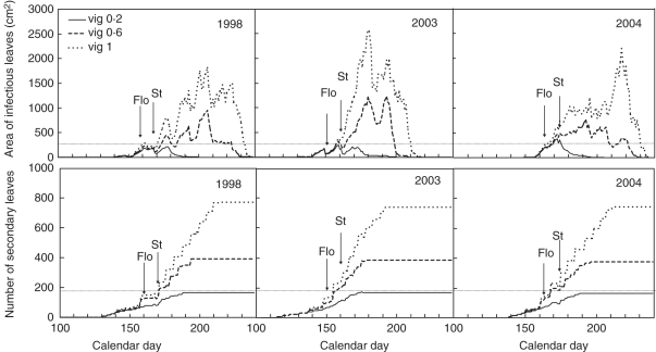
Figure 5 illustrates this, showing that the duration and dynamics of infectious (sporulating) tissue may vary considerably depending on the development of secondary shoots and hence on vigour modulated by the climatic conditions.
Fig. 5.
Simulation of the dynamics of the infectious surface and of the number of secondary leaves as functions of vigour (0·2, 0·6 and 1) and climatic conditions (1998, 2003 and 2004). Flo, flowering; St, shoot topping.
The model thererefore strengthens experimental results observed with regard to the effect of the rate of leaf emergence and of the number of leaves at flowering on the severity of the disease (Valdes, 2007). However, the model also underlines strong variations of the dynamics of leaf emergence depending on the vigour and on the temperature, and therefore on the climatic scenarios that may have various consequences on the damage on bunches of grapes. Further experiments are needed to explore the relationship between vine growth and disease development (a) to demonstrate whether disease development is only controlled by leaf number or also by variation in leaf susceptibility and (b) to test which crop management system could be easily feasible to improve the disease control level.
A continuous simulation model
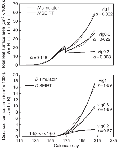
Overall, the total foliar area time dynamics are well approximated by the logistic growth and parameters estimated both before and after shoot topping (Table 1, Fig. 6) with some variations depending on the year. As an example, for 2003 the strong increase in leaf surface after shoot topping corresponding to the higher rate of secondary leaf emergence is well described and yields a higher rate of host growth compared with the other years. However, obviously in the extreme case of a year with an early fast growth followed by a slower rate of increase and then again a fast growth of the foliar surface (i.e. 1998), the fitting is not so accurate. The various levels of vigour, enhanced after shoot topping, are well represented by strong differences in the values of the growth rate parameter, with variations by a factor of 10 between vigour 0·2 and vigour 1.
Table 1.
Parameters of host growth and disease transmission estimated for the SEIRT model by fitting to the daily leaf surface and diseased surface from the mechanistic model
| Year | Vigour level | Parameters for host growth |
Parameters for disease transmission for early inoculation |
Parameters for disease transmission for late inoculation |
|||||||||||||||
|---|---|---|---|---|---|---|---|---|---|---|---|---|---|---|---|---|---|---|---|
| Before shoot topping |
After shoot topping |
Before shoot topping |
After shoot topping |
Before shoot topping |
After shoot topping |
||||||||||||||
| α | Nst | J | α | Nend | J | r | Dst | J | r | Dend | J | r | Dst | J | r | Dend | J | ||
| 2004 | 1·0 | 0·147 | 21700 | 2·1 × 105 | 0·032 | 58500 | 2·6 × 106 | 1·605 | 1400 | 202 | 1·688 | 17 150 | 3·4 × 105 | 1·50 | 7·57 | 0·10 | 3·01 | 3264 | 1·18 × 104 |
| 0·6 | 0·148 | 20300 | 1·6 × 102 | 0·022 | 36370 | 2·6 × 106 | 1·559 | 1120 | 155 | 1·690 | 9740 | 2·7 × 105 | 1·46 | 6·62 | 0·11 | 2·10 | 386 | 50·4 | |
| 0·2 | 0·148 | 18560 | 1·7 × 105 | 0·003 | 15481 | 2·5 × 104 | 1·535 | 979 | 199 | 0·669 | 2393 | 4·2 × 104 | 1·48 | 6·61 | 0·16 | 1·94 | 59·7 | 0·8 | |
| 2003 | 1·0 | 0·142 | 20000 | 2·0 × 106 | 0·066 | 84500 | 3·4 × 106 | 1·585 | 1050 | 859 | 2·466 | 41 190 | 1·1 × 106 | 0·86 | 7·00 | 0·20 | 3·80 | 21000 | 1·3 × 106 |
| 0·6 | 0·145 | 17600 | 1·8 × 106 | 0·042 | 50650 | 2·9 × 106 | 1·571 | 913 | 955 | 2·351 | 20 310 | 3·4 × 105 | 0·85 | 6·20 | 0·06 | 3·32 | 6060 | 1·8 × 105 | |
| 0·2 | 0·147 | 16000 | 1·2 × 103 | 0·005 | 17420 | 8·8 × 104 | 1·551 | 785 | 1190 | 1·009 | 2630 | 2·1 × 104 | 0·86 | 6·11 | 0·07 | 4·39 | 421 | 3·8 × 103 | |
| 1998 | 1·0 | 0·174 | 15540 | 5·6 × 105 | 0·037 | 87500 | 8·2 × 106 | 1·602 | 1110 | 1060 | 1·721 | 31 050 | 1·2 × 105 | 1·80 | 24·00 | 0·34 | 2·69 | 22600 | 5·8 × 105 |
| 0·6 | 0·174 | 14600 | 5·4 × 105 | 0·021 | 51000 | 5·1 × 105 | 1·560 | 919 | 766 | 1·627 | 13 460 | 4·2 × 104 | 1·71 | 18·00 | 0·25 | 2·40 | 5300 | 2·4 × 104 | |
| 0·2 | 0·175 | 13700 | 4·8 × 105 | 0·003 | 16300 | 2·8 × 105 | 1·537 | 795 | 573 | 0·378 | 1660 | 3·1 × 103 | 1·71 | 17·30 | 0·25 | 3·50 | 343 | 2·5 × 103 | |
α, rate of host growth (d−1); Nst, total leaf area before shoot topping; Nend, total leaf area at day 210 for 2003, 211 for 2004 and 230 for 1998; J, sum of squared residuals divided by the number of daily outputs minus the number of estimated parameters; r, rate of disease transmission (d−1); Dst, diseased surface area before shoot topping; Dend, diseased surface area at day 210 for 2003 and day 230 for 1998 and 2004.
Fig. 6.
Estimated parameters of the rate of host growth (α) and disease transmission rate (r) and evolution of the total leaf area (N) and diseased area (D) simulated by the mechanistic model and the SEIRT model, before and after shoot topping for the year 2004, and level of vigour 0·2, 0·6 and 1 for early inoculation or late inoculation.
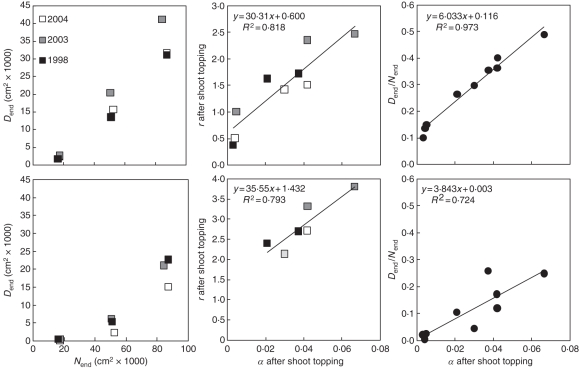
For early inoculation, the diseased surface is also well approximated by the SEIRT model. Before shoot topping, the rate of disease transmission does not vary significantly, but for each year there is a positive linear relationship between r and the disease level at shoot topping (Dst). For a similar rate of disease transmission and rate of host growth, higher levels of disease at shoot topping are due to a higher initial level of inoculum (initial colony size E0; Table 1). Such a higher E0 for 2004, for example, is the consequence of the development of the disease under higher temperature. After shoot topping, we observe a positive linear relationship between α and r and between α and the disease severity Dend/Nend at the end of simulation. This is consistent with the development of secondary leaves with a higher level of disease at the end of simulation for the year 2003 (Table 1, Fig. 7).
Fig. 7.
Relationships between the total leaf area (Nend) and the diseased area (Dend) at the end of the season, the rate of host growth (α) and the disease transmission rate (r) after shoot topping, and the proportion of diseased leaves for the different years and vigour levels 0·6 and 1 at early (top graphs) or late inoculation (bottom graphs) given by the SEIRT model.
For late inoculation, the inoculation occurred at the same phenological stage (four leaves) for each year, but due to different temperature scenarios the time interval between inoculation and shoot topping varies. As a consequence, the rates of disease transmission vary mostly according to the year. The level of disease is very low in the first part of the epidemic. After shoot topping, there is still a positive linear relationship between α and r if vigour 0·2 is excluded. For vigour 0·2, the disease severity is around 2 % and is almost constant. This may explain the difficulty for the model in giving a reasonable value for r.
DISCUSSION
Effect of vine growth on epidemics of powdery mildew
In this article, we illustrated the ability of a complex discrete deterministic model to simulate various levels and dynamics of growth of grapevine with possible high impact on powdery mildew epidemics. Our simulations allowed assessment of the effect of vine vigour on the epidemics and to point out the existence of variations depending on climatic scenarios. Variations between years can mainly be explained by the variations of vine growth rather than the direct influence of the temperature on the pathogen. The positive effect of increased vigour on the disease dynamics had already been experimentally investigated or only pointed out by several authors (Zahavi, 2001; Evans et al., 2006; Valdes, 2007; Calonnec et al., 2009). This increase can be modulated according to the climatic scenario and the effect of temperature on the host growth. The results of our simulations are consistent with the field experiments. The severity of the disease is correlated with the rate of leaf emergence early in the season and the development of secondary shoots later on, combined with the number of infected leaves at flowering. The model, however, indicates that potential variation of vine growth according to the climatic scenario could alter the synchronism between the disease and the production of susceptible organs and possibly delay the severity of the disease. This has an impact on the time evolution of the infectious tissue with potential variations of the damage on bunches of grapes.
Field experiments have been undertaken to explore further whether disease development is only controlled by leaf number or also by variation in leaf susceptibility and to test which system of crop management could better control the disease level. Crop management and modifications of the topological distance between organs can modify assimilate partitioning into the plant (Pallas et al., 2010); this may have an effect on the infection by spores (Goheen and Schnathorst, 1963; Doster and Schnathorst, 1985) and could be used to manage the disease. Leaf susceptibility can easily be modified in the discrete model. We also need to assess the range of sporulation of different powdery mildew isolates. Indeed an intermediate level of vigour attacked by high sporulating isolates could yield the same disease severity as a higher level of vigour and a low sporulating isolates.
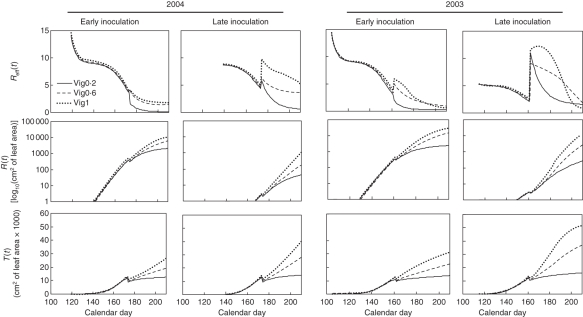
The SEIRT model was able to describe the host growth and the disease dynamics from the outputs of the discrete model during a whole crop season including shoot topping. We obtained a set of parameters for the rate of host growth and the rate of disease transmission with a biological meaning. Different scenarios of vine growth corresponding to contrasting climatic scenarios can be modelled and generate various types of epidemics provided different initial conditions are used (value of E0). For late epidemics starting under higher temperatures, the value of E0 is increased. This value may be deduced from the output of the mechanistic model. The mathematical analysis of the SEIRT model and the simulations of the effective reproductive number Reff (cf. Appendix, Fig. 8) give a synthetic view of the relationship between host growth and the disease. Reff is very high in the case of an early contamination, and decreases during the season, but can increase after shoot topping when the vigour is high, with an increased rate of development of secondary shoots. This increase in Reff after shoot topping differs depending on the climatic scenario.
Fig. 8.
Simulations according to the SEIRT model of the effective reproductive number (Reff), removed foliar surface (R) and immune foliar surface due to ontogenic resistance (T) as a function of time, for the climatic scenario 2004 and 2003 at early and late inoculation.
With this model, it was assumed, however, that the proportion in each compartment does not vary at shoot topping. This may be inaccurate for some climatic scenarios where the tissue growth increases strongly before shoot topping, as in 2004. The transfer of the mechanistic model to the simulation platform OpenAlea (Pradal et al., 2008) would allow better monitoring of the surface and position of the tissues of different ages in the vinestock and therefore better approximation of the temporal evolution of the surface of susceptible tissue, especially after shoot topping. Thus, the SEIRT model may be improved by adding an age structure of the leaves and time since infection for each age. The model would become a PDE model (partial differential equations model) (Webb, 1985). We also observed a linear relationship between α and r, which was unexpected, according to the assumption of true mass action (all sporulating leaves have an equal probability to infect a healthy leaf) where r should be constant. These results suggest that at least one disease mechanism described in the deterministic model is not explicitly taken into account in the SEIRT model (distance between susceptible organs, density-dependent dispersal, etc.) and prevent the use of parameters of plant growth and disease progression independently. There are alternative epidemic models (Ferrandino, 2008) that, although they take into account the canopy filtration (but not the ontogenic resistance), show a reverse relationship between host growth and r. Choosing a true mass action contact term (rather than mass action) and adding ontogenic resistance to the model led to better fits (the sum of squared residuals was lower) than mass action in our experiments. The relationship between r and α could also be linked to the different typologies of host growth, especially to the rate of secondary leaf emergence. A righer rate of host growth after shoot topping means a higher amount of secondary susceptible leaf tissue.
Specificity of the models and perspectives
Our mechanistic model was the first model developed coupling the 3-D dynamics of growth of a plant with those of a pathogen taking into account susceptibility of organs, some types of crop management and the dispersion process. Since then, other models have been developed. For example, a similar model was developed to study the relationship between the dynamics of wheat and the fungus Septoria tritici (Robert et al., 2008). Plants display a wide range of growth dynamics and architectures, so all pathogens are not sensitive to the same climatic variables and may have different dispersion processes. In all these cases, the modelling approach would be useful to test the effect of plant growth and architecture in the epidemic process and later on to predict disease behaviour in the context of climatic changes affecting the plant, the pathogen and their synchrony. This type of model could also be a useful tool to select the most appropriate plant genotypes combining unfavourable characteristics of development and resistance able to maintain the disease at a low level.
Although these deterministic models are interesting in order to understand complex interactions at the scale of the plant or of a few individuals, they are difficult to extend to the plot or larger scale. The SEIRT model using parameters assessed from mechanistic model output is an original way to simplify the modelling without losing the biological and agronomical meaning of the mechanisms described and of the parameters associated which would allow the extension at a larger scale.
To explore the influence of the crop architecture (density of plantation, spatial organization, etc.) and of the heterogeneities within the plot (e.g. vigour) and between plots (e.g. phenology), we will use a spatially structured reaction–diffusion system in the spirit of our earlier work (Burie et al., 2007; Burie and Ducrot, 2009). In this reaction–diffusion model the parameter describing the disease transmission is expressed as a product of the spore's infection efficiency and a rate of production of spores per infectious tissue. The spores can be dispersed at short and long distances. A combination of parameters (infection efficiency, rate of spore production) corresponding to distinct situations of crop growth and pathogen initiations could be tested. We could then explore the conditions of plant growth, densities and resistance (either by cultivars, treatments or delay of contamination) for which the epidemic could be maintained at a low level using, among other things, the effective reproduction ratio (see the Appendix). Already at the vine scale, the behaviour of Reff gives some indications regarding how better to control the epidemic. For example, in the case of an early epidemic when Reff is very high, the only way to control an epidemic may be to spray fungicide on the vines. In the case of late contamination, vigour should be kept low to maintain Reff at a low value. Another way to limit the increase of Reff could be to remove part of the secondary shoots, which is a common practice in high value added vineyards to increase the wine quality.
However, both the mechanistic and the SEIRT models need to be more deeply explored by a rigorous sensitivity analysis performed on parameters from the pathogen, the dispersion and the host susceptibility with variation of the date of inoculation. This sensitivity analysis must be conducted for both models in conjunction since, in particular, the mean duration of the infection i is a parameter used by both models with the same meaning and value and is not easily measured experimentally.
ACKNOWLEDGEMENTS
This study was supported by grants from the ‘Agence Nationale de la Recherche’ programme SYSTERRA (ANR-08-STRA-04) and from INRIA, ‘Action de Recherche Collaborative’ (INRIA M2A3PC).
APPENDIX
Mathematical analysis for the SEIRT model
The basic reproduction number R0 is a threshold dimensionless number that indicates if the epidemic will spread (if R0 > 1) or die out (if R0 < 1); see, for example, Gilligan and van den Bosch (2008). It is defined biologically as the mean number of secondary cases caused by a single infectious individual during its lifetime in a complete susceptible population. For the HLSR model considered by Segara et al. (2001) it is proved that a basic reproduction number R0 exists and its value is:
For our SEIRT model there are two major differences compared with the HLSR model: the foliar surface is not constant and a varying proportion of the healthy foliar surface is not susceptible to the disease. Therefore, as in Cintron-Arias et al. (2009), for example, it is better to consider the effective reproduction number Reff(t). This number depends on time and takes into account the ontogenic resistance to the disease. We can prove that
This number is always lower than R0 since S is lower than N. We can use a simple argument to compute Reff(t): let (E + I) be the ‘active’ diseased foliar surface, adding the second and third equation of the model gives:
Therefore, the disease will die out if Reff(t) < 1 as (E + I)' will be negative and the ‘active’ diseased foliar surface will decrease; conversely if Reff(t) > 1 the disease will start spreading.
Reff(t) = riS(t)/N(t) cannot be computed explicitly for any value of the model parameters. However, if the initial contamination takes place before shoot topping we have S(t0) = N(t0) at bud break and one can prove, using a phase plane analysis employing nullclines [see, for example, Edelstein-Keshet (1988) for a description of the method] that Reff decreases over time whatever the value of the logistic law parameters for growth (Fig. 8). Hence, before shoot topping, a late contamination is less likely to succeed than an early one, and the intensity of the epidemic that follows will be lower. At shoot topping Reff changes depending on the quantity of susceptible and total foliar surface cut, and the previous result is not valid. In particular Reff could increase and reach a maximum value before converging to 0. This must be related to the rate of development of secondary leaves. The value of Reff before shoot topping is dependent on the amount of T.
Next, as time goes to infinity, the solution of the system converges to (0,0,0,R*,T*) with R* + T* = K for any no trivial initial condition and R* > 0, i.e. some foliar surface fraction always remains healthy. The proof is classical and can easily be adapted from that for the spatial model in Burie et al. (2007). Nevertheless, in contrast to the HLSR model considered by Segara et al. (2001) where y∞ = R*/K is the unique solution of equation
and only depends on R0, we could not compute in closed form the final size R* of the epidemic as a function of the model parameters.
LITERATURE CITED
- Analytis S. Obtaining of sub-models for modeling the entire life cycle of a pathogen. Journal of Plant Diseases and Protection. 1980;87:371–382. [Google Scholar]
- Burie JB, Ducrot A. Travelling wave solutions for some models in phytopathology. Nonlinear Analysis Real World Applications. 2009;10:2307–2325. [Google Scholar]
- Burie JB, Calonnec A, Langlais M. Modeling of the invasion of a fungal disease over a vineyard. In: Deutsch A, Bravo de la Parra R, de Boer RJ, et al., editors. Mathematical modeling of biological systems: epidemiology, evolution and ecology, immunology, neural systems and the brain, and innovative mathematical methods. II. Boston: Springer; 2007. pp. 11–21. [Google Scholar]
- Calonnec A, Cartolaro P, Deliere L, Chadoeuf J. Powdery mildew on grapevine: the date of primary contamination affects disease development on leaves and damage on grape. IOBC/wprs Bulletin. 2006;29:67–73. [Google Scholar]
- Calonnec A, Cartolaro P, Naulin JM, Bailey D, Langlais M. A host–pathogen simulation model: powdery mildew of grapevine. Plant Pathology. 2008;57:493–508. [Google Scholar]
- Calonnec A, Cartolaro P, Chadoeuf J. Highlighting features of spatio-temporal spread of powdery mildew epidemics in the vineyard using statistical modeling on field experimental data. Phytopathology. 2009;99:411–422. doi: 10.1094/PHYTO-99-4-0411. [DOI] [PubMed] [Google Scholar]
- Chellemi D, Marois J. Development of a demographic growth model for Uncinula necator by using a microcomputer spreadsheet program. Phytopathology. 1991;81:250–254. [Google Scholar]
- Cintron-Arias A, Castillo-Chavez C, Bettencourt LMA, Lloyd AL, Banks HT. The estimation of the effective reproductive number from disease outbreak data. Mathematical Biosciences and Engineering. 2009;6:261–282. doi: 10.3934/mbe.2009.6.261. [DOI] [PubMed] [Google Scholar]
- Doster MA, Schnathorst WC. Effects of leaf maturity and cultivar resistance on development of the powdery mildew fungus on grapevines. Phytopathology. 1985;75:318–321. [Google Scholar]
- Eldelstein-Keshet L. Mathematical models in biology. Classics in applied mathematics. Vol. 46. Philadelphia: SIAM; 2005. [Google Scholar]
- Evans K, Crisp P, Scott ES. Applying spatial information in a whole-of-block experiment to evaluate spray programs for powdery mildew in organic viticulture. In: Pertot I, Gessler C, Gadoury D, et al., editors. Proceedings of the 5th International Workshop on Grapevine Downy and Powdery Mildew. San Michele all'Adige, Italy: Instituto Agrario di S. Michele all'Adige; 2006. pp. 169–171. [Google Scholar]
- Ferrandino FJ. Effect of crop growth and canopy filtration on the dynamics of plant disease epidemics spread by aerially dispersed spores. Phytopathology. 2008;98:492–503. doi: 10.1094/PHYTO-98-5-0492. [DOI] [PubMed] [Google Scholar]
- Gadoury D, Seem R, Ficke A, Wilcox W. Ontogenic resistance to powdery mildew in grape berries. Phytopathology. 2003;93:547–555. doi: 10.1094/PHYTO.2003.93.5.547. [DOI] [PubMed] [Google Scholar]
- Gessler C, Blaise P. An extended progeny/parent ratio model: II Application to experimental data. Journal of Phytopathology. 1992;134:53–62. [Google Scholar]
- Gilligan CA, van den Bosch F. Epidemiological models for invasion and persistence of pathogens. Annual Review of Phytopathology. 2008;46:385–418. doi: 10.1146/annurev.phyto.45.062806.094357. [DOI] [PubMed] [Google Scholar]
- Goheen AC, Schnathorst WC. Resistance to powdery mildew in grapevines related to osmotic value and associated factors (abstract) Phytopathology. 1963;53(1139) [Google Scholar]
- de Jong MCM, Diekmann O, Heesterbeek JAP. How does transmission and infection depend on population size? In: Mollison D, editor. Epidemic models: their structure, relation to data. Cambridge: Cambridge University Press; 1995. pp. 84–94. [Google Scholar]
- Pallas B, Christophe A, Lecoeur J. Are the common assimilate pool and trophic relationships appropriate for dealing with the observed plasticity of grapevine development? Annals of Botany. 2010;105:233–247. doi: 10.1093/aob/mcp278. [DOI] [PMC free article] [PubMed] [Google Scholar]
- Peyrard N, Calonnec A, Bonnot F, Chadoeuf J. Explorer un jeu de données sur grille par tests de permutation. Revue de Statistique Appliquée. 2005;LIII:59–78. [Google Scholar]
- Pradal C, Dufour-Kowalski S, Boudon F, Fournier C, Godin C. OpenAlea: a visual programming and component-based software platform for plant modelling. Functional Plant Biology. 2008;35:751–760. doi: 10.1071/FP08084. [DOI] [PubMed] [Google Scholar]
- Robert C, Fournier C, Andrieu B, Ney B. Coupling a 3D virtual wheat (Triticum aestivum) plant model with a Septoria tritici epidemic model (Septo3D): a new approach to investigate plant–pathogen interactions linked to canopy architecture. Functional Plant Biology. 2008;35:997–1013. doi: 10.1071/FP08066. [DOI] [PubMed] [Google Scholar]
- Segarra J, Jeger MJ, van den Bosch F. Epidemic dynamics and patterns of plant diseases. Phytopathology. 2001;91:1001–1010. doi: 10.1094/PHYTO.2001.91.10.1001. [DOI] [PubMed] [Google Scholar]
- Tenenhaus M, Esposito Vinzi V, Chatelinc YM, Lauro C. PLS path modeling. Computational Statistics & Data Analysis. 2005;48:159–205. [Google Scholar]
- Valdes H. Relations entre états de croissance de la vigne et maladies cryptogamiques sous différentes modalités d'entretien du sol en région méditerranéenne. 2007 PhD Thesis. Ecole de Montpellier supAgro, Montpellier, France. [Google Scholar]
- Webb GF. Theory of nonlinear age-dependent population dynamics. (Monographs and textbooks in pure and applied mathematics; 89) New York: M. Dekker; 1985. [Google Scholar]
- Zahavi T, Reuveni M, Scheglov D, Lavee S. Effect of grapevine training systems on development of powdery mildew. European Journal of Plant Pathology. 2001;107:495–501. [Google Scholar]


