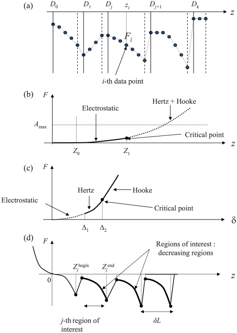
Figure 1. Main notations and schematic illustration for the three steps of the proposed algorithm.

(a) Segmentation of a force curve (first step). The data points (, ), i = 1,…,n are partitioned into k+1 contiguous intervals , …, with and the minimal and maximal values. The plain and dashed vertical lines represent the left and right bounds of the segmented intervals. The experimental data are smoothed on each interval (piecewise smoothing). (b) Detection of the electrostatic region in the -domain (second step) and fitting to the electrostatic model (third step). The critical points and are the edges of electrostatic region in the -domain. A _max is an upper bound for the exponential prefactor A. It is optional but useful for improving the detection of the edge by forbidding -values that lead to unrealistic values of A. (c) Segmentation and fitting in the δ-domain (third step). The critical points  =  and  =  correspond to the beginning of the Hertzian and Hooke regimes, respectively. (d) Retraction curve: the j–th region of interest is the j–th decreasing interval . The search for these regions is done from the outputs of the segmentation algorithm (second step), then the data are fitted to the FJC model within each region of interest (third step).