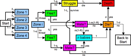
Figure 1.

Probabilistic automaton model of the life cycle of a prey animal. At each time step, every animal begins in the state “start,” and follows a complete path, ending either back at the start, or in death. Each arrow is labeled with the conditional probability that the given event occurs (die, survive, etc.), once the animal reaches the box at the tail of that arrow. The animal spots a potential threat in zone i with probability δ_i. Four zones (groupings by predator–prey distance) are shown in the diagram. The threat is real with probability α. If there is a threat the prey animal flees with probability p_i. Those animals that do not flee are killed with probability L_i, while those that do flee always escape. The animals that neither flee nor die mate with probability m, producing n progeny. The animals that do flee suffer a reduced mating rate of m(1 − R). In order to keep the population stable, some randomly selected animals are killed at the end of the time step with probability σ. The probability of any path is obtained by multiplying the conditional probabilities of each subsequent step. A sample path is illustrated by the dashed arrows in the diagram: The animal spots a potential threat in zone 3. This is not a real threat, but, with its imperfect information, the animal incorrectly decides to flee. It then mates, producing n progeny, which are added to the population for the next time step. The animal does not succumb to disease, starvation, or other non-predation-related causes of death, and lives on to the next time step. The probability of this path is δ₃(1 − α)q_im(1 − R)(1 − σ).