Fig. 2.

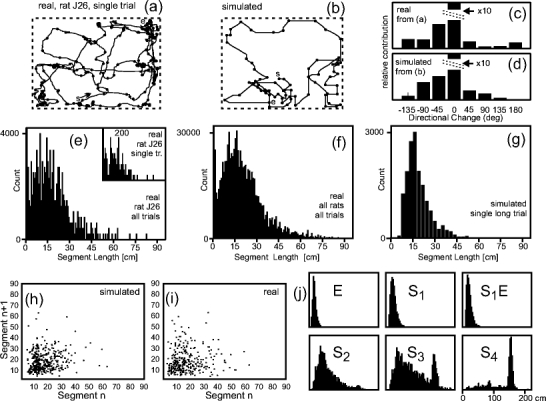
Statistical analysis of real and simulated rat trials. (a) Example of a real rat trial in a rectangular arena. Walls of the arena are shown by the dashed box. Dots mark break points between straight stretches. (b) Simulated trial. Start and end-points are marked (s, e). (c, d) Distribution of turning angles for a real (c) and a simulated (d) trial. (e–g) Distribution of straight stretches for real (e, f) and simulated (g) trials scaled to their individual peak height. Panel (e) shows the distribution of straight stretches for a single rat (all trials), inset in (e) shows a single rat trial as given in panel (a). Panel (f) contains all five experimental sessions with real rats and (g) simulated trial. The simulated path was generated using ‘SE’ strategy (see subsection ‘Path Generation and Exploration Strategies’). Panels (h) and (i) show scatter plots of subsequent path segments. Small panels (j) depict the distributions from trials with different S and E components as shown by the labels. For S1 the default parameters were used, for S2, S3 and S4 we have S2: p1 = 0.8475, p2 = 0.0656, p3 = 0.0087, p4 = 0.0019, p5 = 0, p6 = 0.0019, p7 = 0.0087, p8 = 0.0656; S3: p1 = 0.9386, p2 = 0.0286, p3 = 0.0018, p4 = 0.0002, p5 = 0, p6 = 0.0002, p7 = 0.0018, p8 = 0.0286; S4: p1 = 0.9940, p2 = 0.0030, p3 = p4 = p5 = p6 = p7 = 0, p8 = 0.0030