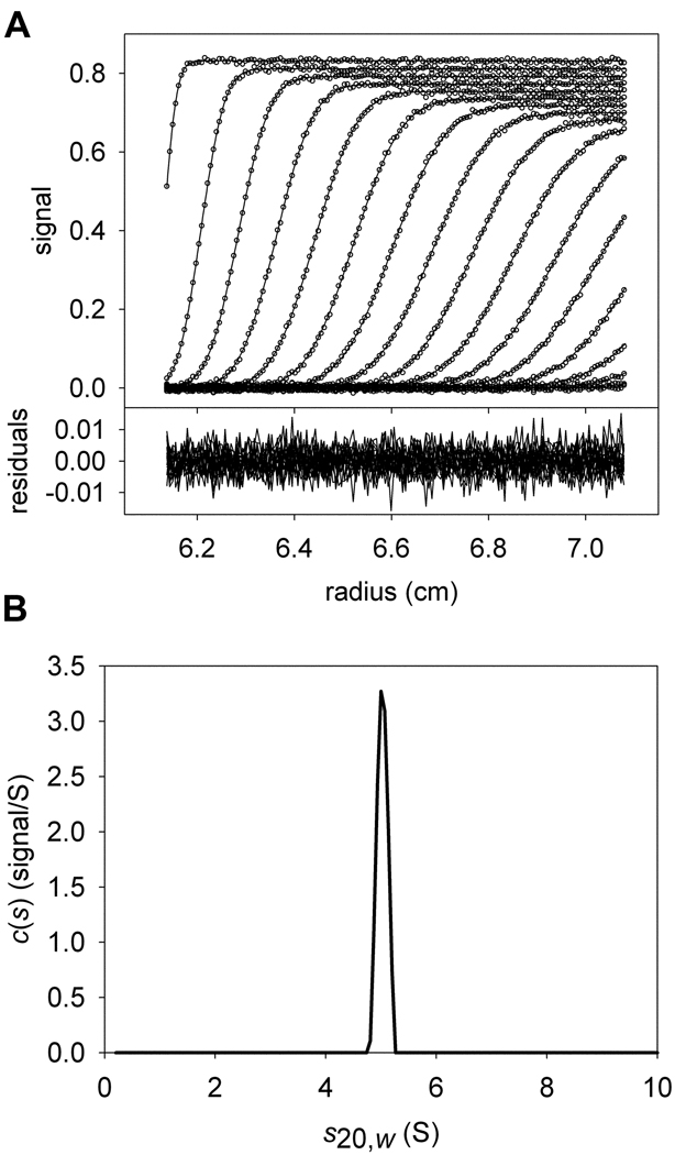
Figure 1. The conventional c(s) distribution.

Conventions established in this figure will hold for all other figures, except where noted. (A) Simulated sedimentation velocity data and fit thereto. In the upper part, the individual data points are represented as open circles; they form the characteristic sigmoid shape that describes one point in time (i.e. a “scan”) during the experiment. The inflection point of this feature moves from left to right as time progresses. The x-axis shows the radius from the center of rotation. The y-axis in the upper part shows the magnitude of the signal. For clarity, only every 6^th data point used in the data analysis is shown. Also, only every 3^rd scan used to analyze the data is shown. The fit to these data using the c(s) distribution in part B is shown as a solid line. The lower part of the figure shows the residuals as a function of radius, where the residual is equal to the y-value of a given data point minus the y-value of the fitted data point. The data were simulated using a single signal (λ1) to include two species (A and B) with identical hydrodynamic characteristics (5 S, 77081 Da), but different concentrations:[A] = 5 µM; [B] = 2 µM; ${\epsilon }_{\text{λ1}}^{\mathrm{A}}={\epsilon }_{\text{λ1}}^{\mathrm{B}}=\mathrm{100,000}$ M⁻¹cm⁻¹. (B) The c(s) distribution that best describes these data. On the x-axis is the s_20,w of the simulated species used for the fit, and on the y-axis is the normalized population of material present for each species. This distribution describes the data well, but no spectral discrimination between the two proteins is afforded.