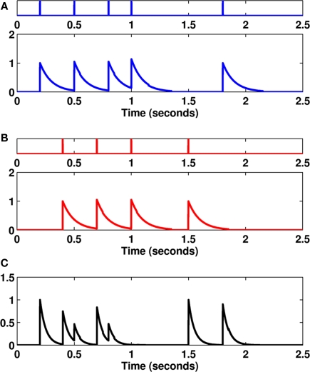
Figure 2.
(A–B) An example of two spike trains (colored blue and red) along with the transformed spike trains f1 and f2 using an exponential kernel function with parameter τ = 100 ms. (C) An example of the squared difference in the transformed spike trains. Evaluating the area under this curve gives us the van Rossum distance between the two spike trains.

