Figure 4.
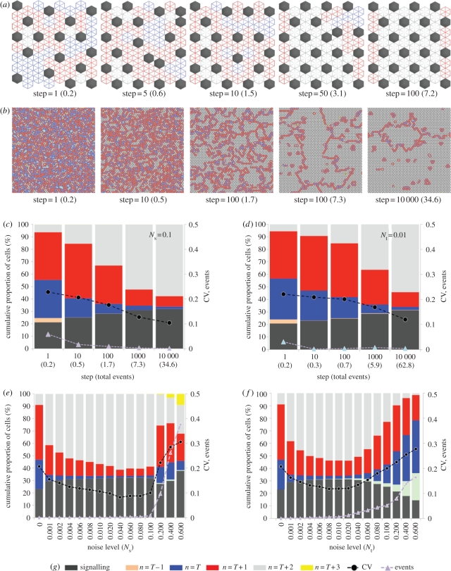
Signal noise leads to pattern optimization. (a,b) Simulations of inhibitory signalling with spatial noise, Ns = 0.1, T = 1, (a) executed in an 8 × 8 hexagonally packed array of cells and (b) a 100 × 100 array of cells with toroidal boundaries. Each image shows the pattern at a particular ‘step’ in the simulation advancing from left to right. A single step represents a number of cell updates equal to the total number of cells in the array. The number shown in brackets represents the total proportion of cells that have switched state (total events). The state of cells is defined by the colour key in (g): dark-grey cells actively express the inhibitory signal and all inactive cells are coloured according to their total number of active neighbours. As the patterns move towards a state of optimized packing this corresponds to a reduction in the number of blue (one active neighbour) and red (two active neighbours) cells and an increase in the number of light-grey cells (three active neighbours). Note that with spatial noise adjacent cells sometimes signal (see steps 5 and 50 in (a)), which causes the shift in the pattern towards the optimized state (compare with optimization under temporal noise in the electronic supplementary material, figure S1). In a large field (b) this leads to the development of relatively stable optimized ‘zones’ with unstable active boundaries, which expand over time. See also the electronic supplementary material, movie 1. (c,d) The change over time in the proportion of each cell type represented as a cumulative percentage (plotted on the left-hand y-axis). Data are averaged over 10 simulations. In (c) the conditions are as described in (b). The results of identical simulations with temporal noise, Nt = 0.01 are shown in (d). In addition, the purple triangles show the number of events occurring at each step. The black circles show the coefficient of variation (CV) in the pattern spacing that was measured by recording the distance between each active cell and its six nearest neighbours and taking the ratio of the standard deviation to the mean. The CV and events are plotted on the right-hand y-axis. (e,f) A comparison of the final pattern state achieved after 10 000 steps with different amounts of spatial noise (e) and temporal noise (f). The figures show the mean values from 10 simulations. Optimized patterns are achieved with noise levels in the ranges 0.001 < Ns < 0.1 and 0.001 < Nt < 0.01. At higher levels of noise, the patterns become unstable, as represented by the significant increase in the number of events. NB: Standard errors (95% confidence intervals) in the mean data displayed in (c–f) were less than 1% (left-hand y-axis) and less than 0.01 (right-hand y-axis) and so were not visible on this scale.

