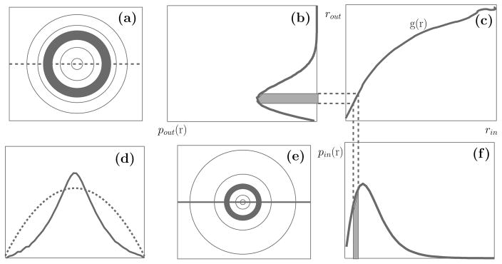
Figure 3.
Radial gaussianization procedure, illustrated for two-dimensional variables. Joint densities of (a) a spherical gaussian and (b) a nongaussian SSD (multivariate Student’s t). Plotted levels are chosen such that a spherical gaussian has equal-spaced contours. (b,f) Radial marginal densities of the joint gaussian and SSD densities in a,e, respectively. Shaded regions correspond to shaded annuli. (c) Radial map of the RG transform. (d) Log marginal densities of the joint gaussian (dashed line) and SSD (solid line) densities.

