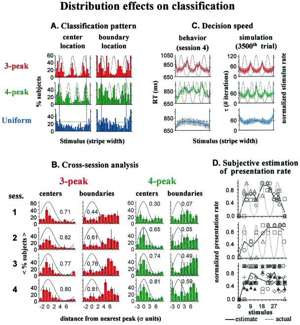
Figure 3.

Stimulus distribution effect on classification. (A) Histograms of class center (Left) and boundary (Right) location for each case, during the fourth classification session, reflecting clear correlation with the statistical pattern of the stimulation in the multipeak cases. Bars of each histogram denote percentage of subjects who had a class center (boundary) at each stimulus. Class center location was computed as the center of gravity of the sorting coherence function, χ, between the two boundaries, i.e., Σb ⋅ χ(b, c)/Σχ(b, c). Dashed lines indicate range of edge effects. (B) Cross-session development of the distribution effect: the center and boundary location histograms of each session are reorganized according to distance from the nearest peak. Bars indicate average percent of subjects locating center or boundary at a specific distance from distribution peak. Error bars denote SD. Numbers are correlations between histograms and the distribution characteristics. Note slower evolution of the effects in the four-peak case. (C) Distribution effect on decision speed. Colored curves indicate cross-subject average behavioral RT data (Left) and simulation convergence time τ (Right). Error bars denote SE and SD of the behavioral and simulation results, respectively. The longer RTs near less frequent stimuli was successfully imitated by the simulation τ. However, τ increased near range edges, where RTs were shorter. (D) Absence of subject awareness of the statistical structure of the stimuli. Dark curves present the cross-subject average subjective rate of presentation frequency (on a five-level scale; normalized between lowest and highest). Data were collected after completion of the classification experiment, where subjects were asked to estimate the frequency of a few serially presented stimuli (usually 15; always including the most and least frequent). Symbols indicate individual estimates. Subjective estimations were not correlated with actual stimulus distributions.