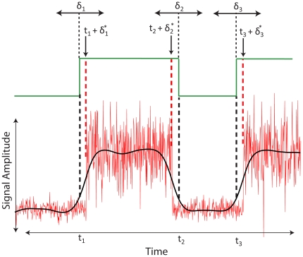
Figure 1. Schematic depiction of the maximum likelihood alignment procedure.

An imaginary ‘two-state’ signal is shown in red. The low-pass filtered observation sequence (black trace) is used to produce the initially decoded Viterbi state sequence (green trace) with state transition times t₁, t₂, and t₃ indicated by the vertical black dashed lines. These transition times are aligned to the broadband observation sequence (red trace) by maximizing the likelihood of a set of perturbations δ_i on the initial state transition times given the broadband observation sequence. Maximum likelihood values of the aligned transition times are then given by the set of times {t_i+δ_i*}, indicated by the red vertical dashed lines. For the signal features used in the majority of the analysis, perturbations of up to ±150 ms were determined to be sufficient; however when exploring a large range of filtering parameters we allowed perturbations of up to ±300 ms on the state transitions.