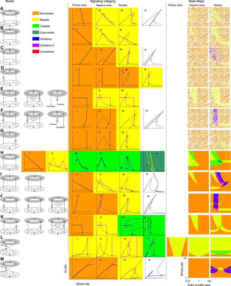
Figure 4.

Many system properties emerge from combinations of signaling and trafficking. Left column shows the model schematic, with one to three cases that obey the same equations. Middle columns show different signaling categories as M versus Mtot curves, along with example solutions. Tick marks on graph axes are at 1 μM intervals. Solutions are also shown from numerical computation of steady states, using dots for stable solutions and open circles for saddles and unstable solutions. Graphs are color-coded to indicate the solution class. Oscillatory solutions (blue) are indicated by blue lines on a white background; the rest have the indicated color as background. All graphs are for compartment A, except for panel J(i–iv)), which is for compartment B, and panel (K iv), which shows how solutions from compartment A in K iii map to compartment B. State maps are shown in the rightmost three columns for positive slope, negative slope, and bistable systems, respectively. These maps indicate by color code the system states that occur for various levels of Mtot (y axis) and ratio of trafficking rates (x axis). The positive slope cases were all singly stable, except for panel L, and were therefore left blank. State map generation is explained in the Methods in the Supporting Material.