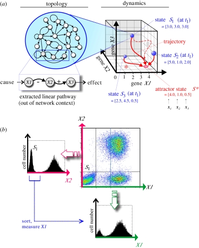
Figure 1.
Schematic of the three perspectives discussed in this paper. (a) From gene-regulatory network topology to dynamics in the state space (§2). The traditional paradigm of a linear pathway as a chain of causation consisting of genes X1, X2, X3 extracted out of the network context is shown as a contrast underneath the network topology map. On the right, a three-dimensional state space capturing the dynamics of a hypothetical three-gene network (genes X1, X2 and X3) is shown. Any point in this space represents a (theoretical) network state S at time t, defined by the expression values x of the sub-network's three genes, S = (x1, x2, x3) (gene-expression pattern) at time t. Three arbitrary states (blue balls), S1, S2 and S3 are shown. Their gene-expression patterns (x1, x2, x3) are indicated and, by acting as the space coordinates, define the position of the states in the state space. Since, as most states, they do not represent stable network states, they are driven by the network interactions to seek a stable state; hence they move in state space along trajectories (red solid lines) that lead to the stable attractor state. The trajectory denoted by asterisk (*) best represents the movement of the state discussed in the main text that manifests the regulatory relationship ‘X1 inhibits X2’—however, it is modulated by other inputs from the network. The dashed trajectory represents an example of a trajectory that has been perturbed (e.g. by drugs that affect expression of genes X1, X2 and X3) away from its natural course defined by the network interactions into regions of the state space that are even less stable, and hence quickly returns to the trajectory that leads to the attractor. In summary, the states, S1, S2, S3 and the perturbed trajectory all lie within the state-space region that ‘drain’ to the particular attractor S*, hence they all lie within its basin of attraction. (b) Illustration of both neglected (‘hidden’) dimensions (§3) and heterogeneity of clonal populations (§4). A typical two-dimensional flow cytometry dot-plot output (for hypothetical proteins X1 and X2) with three subpopulations is shown, along with the separate histograms of the projection on the two individual dimensions X1 and X2 (schematic, from simulations). Note that subpopulation S1 (which may represent an attractor with respect to protein X2) when sorted and probed for protein X1 is actually bimodal with respect to the latter.

