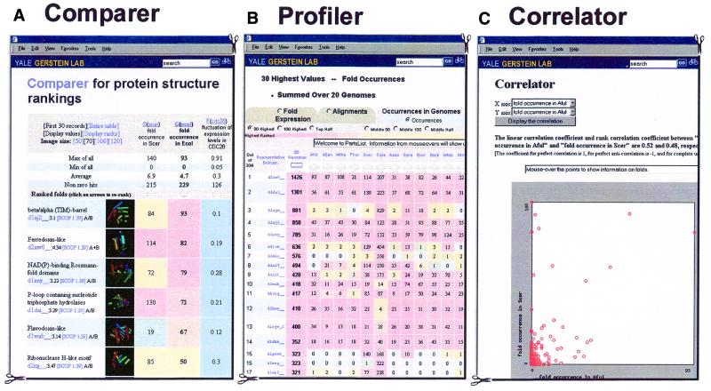
Figure 2.

Sample displays. (A) A sample Comparer display: the four selected attributes are the fold genome occurrence in yeast, the analogous quantity for E.coli, fluctuation of expression level for CDC28 synchronized yeast cell during the cell cycle, and the corresponding values for E.coli to heat shock. (Using the nomenclature in Table 1 these quantities are G(scer), G(ecol), F(cdc28) and F(heatec).) The folds are ranked in terms of fold occurrence in E.coli and the most common fold here is the TIM-barrel (represented by the SCOP domain d1aj2__). If one clicks the ‘Display ranks’ button, the values in the cells will be replaced by the ranks in their respective columns. By clicking the ‘re-rank’ arrows, one can also obtain other views by sorting on other attributes. (B) Shows the occurrences of folds in 20 genomes in Profiler. (C) Shows the correlation between the fold occurrences in the A.fulgidus and S.cerevisiae genomes [G(aful) and G(scer)]. Both linear and rank correlation coefficients are calculated. The linear correlation coefficient is defined as: R = [1/(N–1)]X·Y, where X and Y are two vectors with N elements. Each element of the X vector is normalized thus: X_i = (X_i′ – X)/σ_x, where X and σ_x are the average and standard deviation of the values of the original data vector X′, respectively. Y is normalized in a similar fashion. For two perfectly correlated datasets, R = 1, while for two completely uncorrelated datasets, R = 0. If we replace X_i by its rank among all the other X_i in the sample (i.e., 1,2,3 … N), then we get the rank correlation coefficient. A scatter plot is also shown to help in visualizing this correlation.