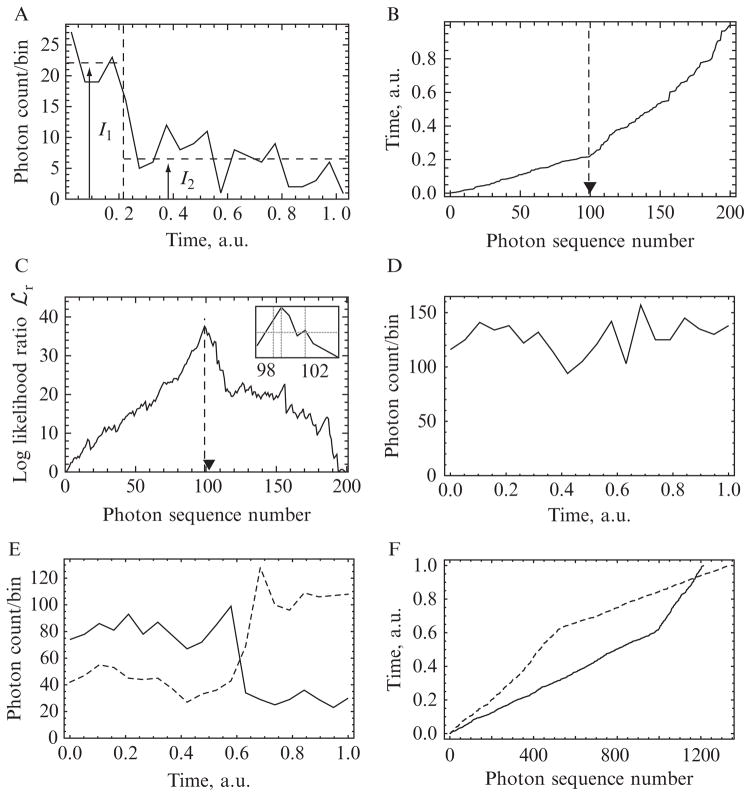
Figure 15.1.

(A–C) Illustration of changepoint detection methods on simulated data with N = 200 photons and a ratio between the high and low rates of χ = 3. (A) The photons are binned into 20 constant-width temporal bins. Examining the graph by eye, we may guess that there is a change in photon rate somewhere around the vertical-dashed line, but neither this change time nor the initial and final rates (I₁ and I₂), nor even the existence of a changepoint, are clear. (B) As described in Section 1.3, the kink in the cumulative distribution of photon arrival times gives a much clearer indication of changepoint time, and the two slopes flanking that point yield the corresponding photon rates. Because these are simulated data, we can compare the actual (triangle) and inferred (dashed line) changepoint times. This chapter describes a quantitative implementation of this simple observation. (C) The peak of the log-likelihood surface occurs at photon sequence number m = 99 (vertical-dotted line), and the 95% confidence intervals at m = 98 and 102 enclose the actual changepoint (inset, vertical lines). (D–F) Illustration on real experimental data. A bifunctional fluorescent dye molecule was attached to one of the two lever arms of a myosin-V molecular motor. The motor bound to an immobilized actin filament and began its mechanochemical cycle in the presence of 10-μm ATP. The dye was excited by polTIRF in each of the several incident polarizations (see Section 2.1), and individual emitted photons were detected after passing through a polarization splitter. (Time-stamped data also arise in FRET measurements.) (D) shows the photon counts in a set of 20-time bins (total of N = 1280 photons recorded). No changepoint is visible to the eye. (E) separates the total counts into the several “flavors,” or tagged subpopulations, of emitted photons. Of these, two have been selected for display as solid and dashed curves. A changepoint is visible, but its time cannot be established to greater accuracy than about two time bins. (F) shows the cumulative distribution described in Section 1.3. Each photon time series displays a sharp kink, and moreover, the two curves’ kinks occur at the same time (vertical position).