Figure 1.

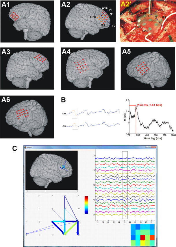
Recording and analysis of SWA propagation. A, Estimations of the positions of recording sites on standard human brain images based on intraoperative photographs and postoperative structural MR images (A1–A6 correspond to Pts. 1–6, respectively). A2′, Photograph taken during the operation. Marked points and electrodes are also exhibited in the corresponding reconstruction image (A2). Recording sites visible in A2′ are displayed in orange in A2. Channel 18 in Pt. 2 as well as channels 5, 17, and 18 in Pt. 6 were dysfunctional (i.e., either no data were recorded by the electrode, or a disproportionate amount of nonbiological noise showed the malfunction of the contact site) and thus left out from the analysis. B, Filtered (0.1–40 Hz) ECoG data were subjected to MI analysis for all pairs of recording channels (see Materials and Methods). One-second-long data segments were compared with time-lagged data from the other channel and the extent of nonlinear correlation (predictability) was measured by MI. Left, Short data segments from two ECoG channels (Ch). Gray shading designates examples of 1-s-long temporal windows for MI calculations. Right, MI was displayed as the function of time lags (1 ms resolution). A significant maximal MI (in this case, 2.61 bits at 153 ms temporal delay) was considered to be a sign of significant correlation between the two channels, which corresponded to propagating sleep slow waves (see Materials and Methods and Results). Left, Time lag between the data windows (gray) was set to the optimal delay (153 ms) at the given time point. Note the similarity of slow-wave cycles (orange) in the windows. This analysis was repeated for all fixed time instances and for all pairs of recording channels. C, Based on the MI analysis, SWA propagation time, distance, and association strength could be assessed for all significant unitary propagation events, from which a time-resolved propagation map was drawn and visualized in a custom-built graphical user interface. A screenshot from this interface is shown with all ECoG channels (top right), amplitude map [bottom right; coldest/warmest color correspond to smallest/largest ECoG amplitude (color bar); 5 × 4 squares correspond to the 5 × 4 grid electrodes; amplitude was calculated as the difference of maximal and minimal ECoG value in the data window], propagation map displayed in a schematic form (bottom left) and also projected to the brain surface (top left). For every time point, arrows on the propagation map designate unitary propagation events between two recording sites (marked by numbers on the schematic view). The color of each arrow shows association strength (warmer colors are stronger) and the width corresponds to propagation time (thicker lines show shorter time).