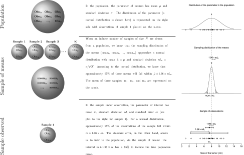
Fig. 2.
The cascade from the distribution of the parameter in the population, to the sampling distribution of the means, and to a single sample is shown. We can see how we work our way back from the mean and standard error of the mean in the sample (m1 = 7.4, and se = 0.57), to construct an interval (m1 ± 1.96 × se), closely resembling the interval  ± 1.96 × sdm, that has a 95% probability to include the true population mean (μ = 8).

