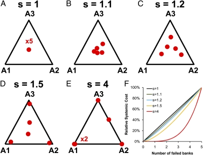
Fig. 2.
Lowest expected cost configurations for different levels of cost function nonlinearity s. (A–E) We consider five banks investing in three assets, with losses drawn from a student t distribution with 1.5 degrees of freedom having a mean = 0 and a 10% chance of being great than the banks' failure threshold of 1. Shown is the lowest expected cost allocation of 105 randomly selected allocations over 106 loss samplings. As s increases, the lowest expected cost configuration moves farther from uniform diversification. The cost function for various values of s is shown in F.

