Figure 17.

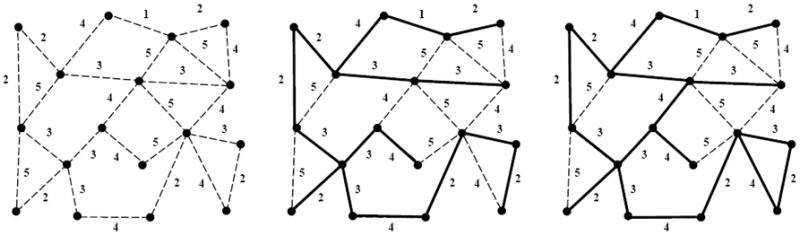
Example of a weighted graph and the resulting minimal spanning tree, as adapted from Ref. [61]. (a) Shows all of the edges and nodes in a graph, with the weight of each edge indicated next to the edge. Graph edges are depicted by broken lines. (b) Shows the minimal spanning tree for this graph, which is the set of edges that connects every node in the graph in the tree with the lowest total weight. Edges included in the tree are shown as solid lines, while edges not included remain broken lines. The total weight of the tree in (b) is 40, and the occupied edge density (number of edges included in the tree divided by total number of edges in the graph) is 15/25 = 0.6. (c) Shows the invasion percolation network for the same graph. Note that the invasion percolation network may have loops and in this case there are two closed loops. If loop formation is prevented (resulting in the highest weight edge in any loop remaining unoccupied) the result is the acyclic invasion percolation network. As can be readily seen by comparing figures (b) and (c) the acyclic invasion percolation network is identical to the minimal spanning tree.