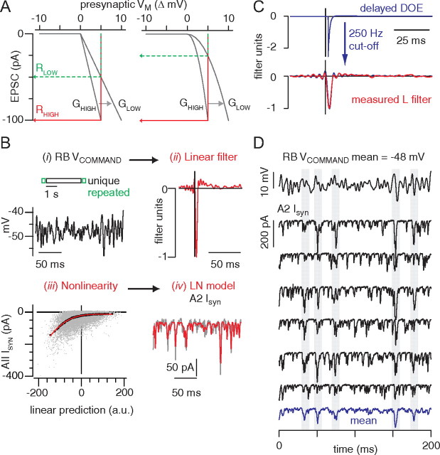
Figure 4.

Linear–nonlinear model for characterizing the RB–AII synapse. A, Schematic representation of the synaptic transfer function between presynaptic membrane potential and postsynaptic current. In both cases, synapse is partly rectifying (zero for potentials negative to rest) and otherwise linear (left) or nonlinear (right). Both a high-gain (G_HIGH) and low-gain (G_LOW) condition are shown; gain in the G_LOW condition was scaled by 0.5 (i.e., ordinate values are plotted against abscissa values multiplied by 2). Response to a +5 mV test pulse from baseline (0 mV) in the low-gain (R_LOW) and high-gain (R_HIGH) conditions are shown. Measuring gain by the ratio R_LOW/R_HIGH yields a correct 0.5 change in the linear case (A1) but an incorrect 0.25 change in the nonlinear case (A2); measuring the complete input–output function using the L-N analysis enables a scaling procedure to reveal the correct gain change in both cases (see Materials and Methods). B, The RB was stimulated with a voltage command (48 ± 3 mV) that included both repeated sequences (350 ms) and a unique sequence (4 s). A single trial is represented schematically, and a representative sample of the repeated stimulus is illustrated below. Trials were separated by 20 s. The L-N model was generated from the unique sequences and tested on the repeat sequences (i). The unique response is convolved with a linear filter (ii) to generate a linear prediction of the AII output (given in arbitrary units). This prediction is passed through a static nonlinearity (iii), characterized by strong inward rectification, to generate the L-N model of AII output. The predicted L-N output (iv) resembles the measured synaptic current (AII I_syn; averaged across six repeats; r² = 0.57 ± 0.07 for n = 5 recorded pairs). The nonlinearity shows the raw data (gray points, downsampled to 1 kHz), the binned data (black points, 200 bins), and the fit compared with the averaged response to the repeated stimulus (red line). C, The measured filter is approximated by a delayed DOE after applying a 250 Hz cutoff (fitted parameters: t_d = 2.0 ms; κ₁ = 2.6; σ₁ = 1.0 ms; κ₂ = 0.05; σ₂ = 26.6 ms). The entire L-N analysis was restricted to frequencies <250 Hz, and the measured filter was used to generate the linear prediction in B. D, Six responses to the repeated stimulus are shown to illustrate the variability of the synaptic responses. This variability gives rise to the scatter evident in the raw data (gray points) binned to generate the nonlinearity in B. The gray bars highlight responses to relatively large depolarizations; these are reproduced with considerable variability from trial to trial.