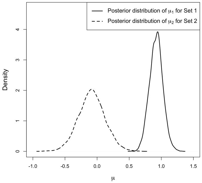
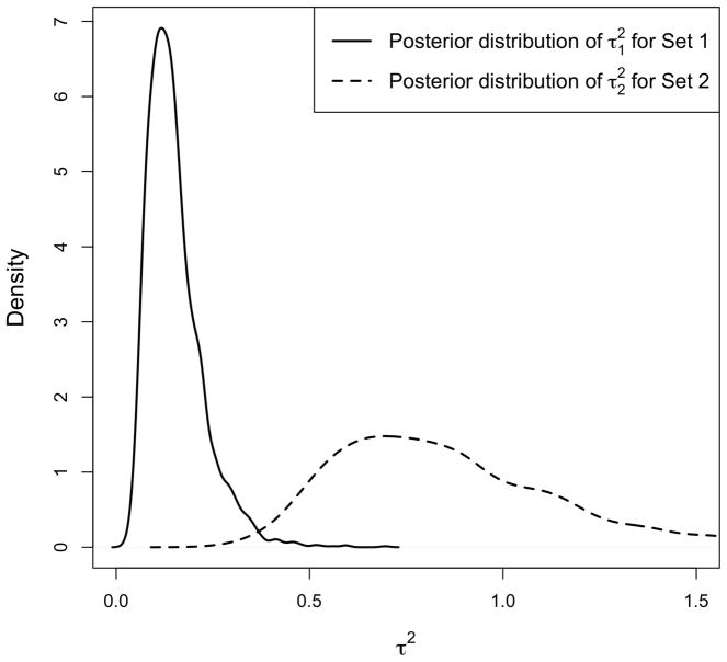
Figure 4.

Posterior distribution of hyperparameters, μ_s and ${\tau }_s^2$, if we assume ${\beta }_{sg}\sim N({\mu }_s,{\tau }_s^2)$. The simulated data includes two gene sets, each with 20 genes. For the first gene set, we set the actual values of β_sg to 1, for g = 1, …, 20. For the second gene set, β_sg is set to −1 for half of the genes and to 1 for the remaining genes. The left panel shows the posterior distribution of μ₁ and μ₂ for Set 1 and Set 2. The right panel shows the posterior distribution of ${\tau }_1^2$ and ${\tau }_2^2$ for the two sets. Notice that the location shift in the distribution of β_sg for Set 1 is captured by μ₁, while the relatively larger variance of β_sg for Set 2 is captured by ${\tau }_2^2$.