Figure 14.

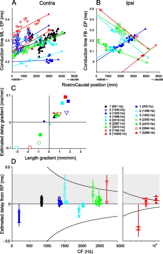
Rostrocaudal gradients of conduction time. A, B, Relationship between estimated conduction time and location of EP in rostrocaudal dimension in contralateral (A) and ipsilateral (B) fibers. The abscissa is zeroed to the position of the most rostral section in which MSO could be identified, and abscissa values are the distance of endpoints to that most rostral section. Ordinate values are the estimated conduction times from the midline (A, contralateral projections) or first branch point (B, ipsilateral projections). Solid lines are linear regressions. The asterisks at the end of each line indicate the most caudal MSO section. Note that the ordinate in B has a wider range than in A. C, Summary of regression slopes of Figure 8, A and B (abscissa), and of A and B (ordinate). Large symbols indicate values that are significant for both abscissa and ordinate. Contra 4 showed significance (p < 0.05) for length but not for delay; and vice versa for Contra 9. D, Relationship between estimated delay and CF. The anchor point of each colored vertical line at 0 delay represents the RP of the MSO. The opposite end shows the extrapolated delay at the CP (corresponding to the delay accumulated between RP and the asterisk in A and B). The small horizontal bars show the range of delays of the linear regression over which endpoints are present. Symbols and lines at positive delays, in the shaded region, are for fibers with a pattern consistent with the trend observed by Yin and Chan (1990); these are the fibers with positive slope in A or negative slope in B. Symbols and lines at negative delays are for fibers with an opposite branching pattern (negative slope in A or positive slope in B). Hyperbolic curves indicate the π limit (i.e., the extent of one period equaling CF⁻¹). The scale of the abscissa is linear in the left panel and logarithmic in the right panel.