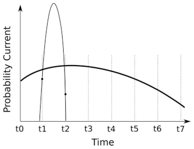
Figure 1.

Illustrative example of the numerical computation of the first passage time probability density function. Time is discretized into t₀, t₁, t₂ … (dotted vertical lines). For a high noise level, the probability current φ varies slowly across multiple bins (bold line) while for low noise, φ varies fast (thin full line). To calculate the FPTPD (see equation 2.3), the gaussian method evaluates the function φ at times t₀, t₁, t₂ … (the intersection of the dotted lines with the φ curve). This is a good approximation for the broad probability current, since it changes slowly within each time bin. In the low-noise case (sharp peak), however, this yields a poor estimate. In the example shown, the value of φ is estimated by the values at t₁ and t₂ (filled circles), which in this case under-estimates the FPTPD. In contrast, the erf method proposed in this study uses the fact that, independent of the discretization, the mean probability current (φ̂) in a bin can be computed analytically. Note that the gaussian method can be improved only with finer discretization; higher-order approximations for the integral will not substantially improve accuracy.