Figure 2.
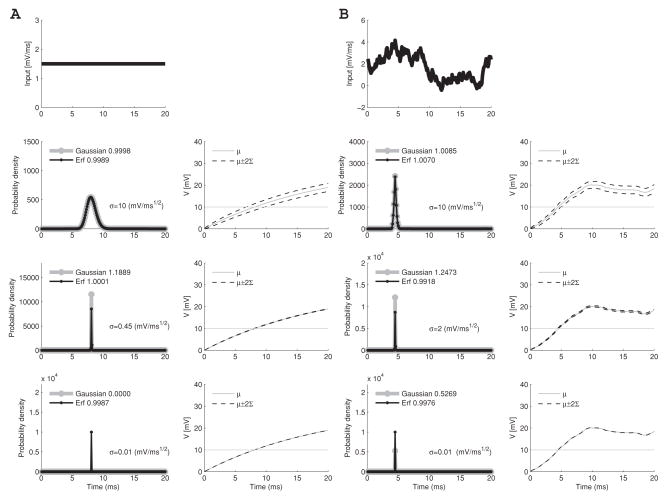
Model behavior at different noise levels for a time interval of length 20 ms, bin width 0.1 ms, and membrane time constant, 1/g(t) = 20 ms. (A) The neuron receives constant input. (B) The neuron receives exponentially decaying impulses from a realistic spike train (see text). The input is shown in both cases in the top row. The lower three rows show, for high (row 2), intermediate (row 3), and low (row 4) noise levels, the first passage time probability density on the left and the mean voltage μ(t) (gray full lines) with its standard deviation Σ(t) (black dashed lines) on the right. The threshold voltage (Vth = 10 mV) is shown by a horizontal line. The likelihood functions (in the left-most panels) are shown in gray lines for the gaussian method and black for the erf method. The integrated value of the FPTPD is shown in each legend; the correct value is unity in all examples. The gaussian method can either overestimate or underestimate the probability density when σ is small.

