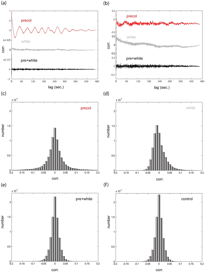
Figure 4. residual analysis.
(a) Results of residual analysis (channel 23, participant 5). In red: the empirical autocorrelation of the residuals after fitting the time series with an SPM HRF model with precoloring. In gray: the results of similar analysis, this time using whitening (see Methods section 2.3). In black: the results using both. In this example, while whitening substantially outperforms precoloring, it is nevertheless improved upon by the combined approach. (b) Results of residual analysis (channel 46, participant 5). Same notation as (a). In this example, precoloring actually outperforms whitening, but again the combined approach is superior to both. (c–f) A histogram of all residual autocorrelation values (lag>0) for this participant using (c) precoloring (d) whitening (e) both. (f) histogram of all residual autocorrelation values (lag>0) resulting from applying the same design matrix with OLS to white noise. As shown, the combined the FGLS approach we propose is very close to the theoretical limit of efficiency.

