Figure 3.

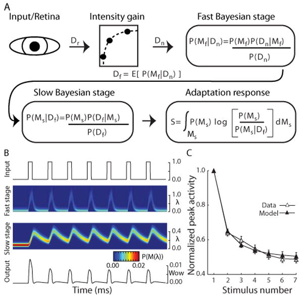
A. Schematic of the Bayesian adaptation model. Light stimulating the retina was modeled as a square wave of unity amplitude (D_r; 1.1 and 0.9 for the brighter oddball conditions) and passed through a static gain function that was constant for all model neurons (see Methods). Two stages of Bayesian learning supply the adaptation dynamics. In each stage (subscripts omitted), the learning process builds hypotheses or beliefs (probability distribution) over a class of internal models M that represent all possible values of its input. As new sensory data D_r is collected, Bayes theorem provides the mechanics to turn a prior set of hypotheses P(M) about which model best characterizes the input data into a posterior set of hypotheses P(M|D), given the likelihood of the data P(D|M) under the assumptions of model M. The fast Bayesian stage quickly adapts to the input and passes the expectation of its posterior beliefs D_f as input to the second Bayesian stage. A posterior set of beliefs is computed in the same fashion as the fast learner, but with a slower learning dynamic. The adaptation response is then calculated for every data observation as the Kullback-Leibler (KL) divergence (Kullback, 1959) between the slow learner's prior and posterior hypotheses, signaling the amount of shift in the model's beliefs caused by each new observation. B. Detailed view of the model dynamics across each stage during a control trial (see methods for a detailed description of the model). Top trace represents the input stimulus from control trials. The two central images show, for each Bayesian learner, the distribution of beliefs about which of the possible Poisson firing rates (y-axis) best characterizes the input over the course of a single trial (x-axis). Hotter colors indicate that, at a given point in time, there is a higher belief (probability) in a particular firing rate. The bottom panel shows the final output of the system. C. Population mean and standard error of the model (filled symbols) and neural (open symbols) normalized peak responses to the 7 stimuli in the control condition.