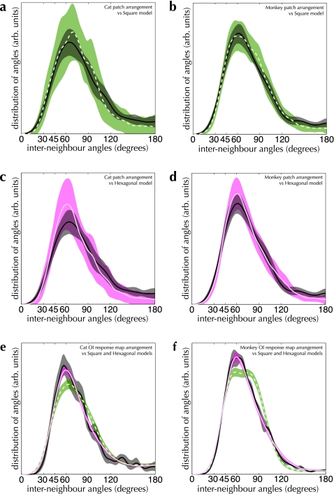
Figure 10.
Comparison between angle distributions from OI response maps, patch-labeling experiments and lattice models. Distributions measured from the indicated experimental dataset are shown as solid black curves and dark shading in all graphs. (a and b) Interneighbor angle distributions measured from patch-labeling experiments (solid black curve and dark shading) compared with a square lattice model (dashed green curve and green shading). In cat area 17 (a), these distributions are significantly different (PK–S < 0.001), while in monkey V1 (b), these distributions are marginally similar at a significance level of α = 1% (PK–S = 0.01). (c and d) Patch-labeling experiments (solid black curve and gray shading) compared with a hexagonal lattice model (solid magenta curve and shading). In cat area 17 (c), these distributions are indistinguishable (PK–S = 0.70); the same is true in monkey V1 (d; PK–S = 0.68). n = 13 injections in a and c, n = 27 injections in b and d. (e and f) Angle distributions measured from OI response maps (solid black curves and gray shading) compared with hexagonal (solid magenta curves and shading) and square (dashed green curves and green shading) lattice models. In both cat area 17 (e) and monkey V1 (f), the square lattice model differs significantly from the OI response map distributions (PK–S < 0.01 for both cat and monkey primary visual cortex). In both cases, the hexagonal lattice model cannot be distinguished from the OI response map distributions (PK–S = 0.10 for cat area 17, PK–S = 0.28 for monkey V1). n = 266 response maps in e, n = 16 response maps in f. 1000 bootstrap resampling runs were performed to estimate the 90% CIs of each of the distributions (shaded regions in all graphs).

