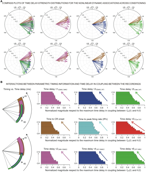
Figure 6.

(A) The compass plots of time delay–strength distributions for the non-linear dynamic associations across the 10 conditioning sessions. In this representation, the time delay–strength distributions (1) [τ1_〈EMG|MN〉, η1_{max 〈EMG | MN〉}] and (2) [τ2_{〈MN | EMG〉}, η2_{max 〈MN | EMG〉}], see magenta arrows, (3) [τ3_{〈EMG | IP〉}, η3_{max 〈EMG | IP〉}] and (4) [τ4_{〈IP | EMG〉}, η4_{max 〈IP | EMG〉}], see blue arrows, and (5) [τ5_{〈MN | IP〉}, η5_{max 〈MN | IP〉}] and (6) [τ6_{〈IP | MN〉}, η6_{max 〈IP | MN〉}], see green arrows, were plotted using the circular statistics method for the inter-stimulus interval of 270 ms (CS–US interval). The 10 colored arrows (10 conditioning sessions, C01–C10) in each circle illustrate the circular dispersion of the angular datasets represented. The two rows of circles show the time delay–strength distributions to explore the time–strength dispersion patterns across conditioning (see the dispersion parameters in Table 3). (B) Interactions between parametric timing information and time delays in coupling between the recordings. The colored circular sectors illustrate the time-dispersion range of the data distributions represented in (A) (see the dispersion parameters Table 2).The colored histograms show the normalized mean values of timing/time delay components of the distributions with respect to the maximum time delay in coupling between f_IP(t) and θ(t) [i.e., the maximum values of τ0_{〈f IP | θ〉} across conditioning sessions].