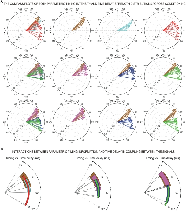
Figure 7.
(A) The compass plots of both parametric timing–intensity and time delay–strength distributions across the 10 conditioning sessions, and for the simulated time condition *ISI = 360 ms. In this representation, the timing–intensity distributions (1) [time to CR onset, percentage of CR], see brown arrows, and (2) [time to peak firing rate of the IP neurons, IPn peak firing rate], see cyan arrows, and the time delay–strength distributions (3) [time delay in coupling τ0〈f|IP|θ〉, maximum linear correlation coefficient rmax〈f IP | θ〉], see red arrows, (4) [τ1〈EMG | MN〉, η1max 〈EMG | MN〉] and (5) [τ2〈MN | EMG〉, η2max 〈MN | EMG〉], see magenta arrows, (6) [τ3〈EMG | IP〉, η3max 〈EMG | IP〉] and (7) [τ4〈IP | EMG〉, η4max 〈IP | EMG〉], see blue arrows, and (8) [τ5〈MN | IP〉, η5max 〈MN | IP〉] and (9) [τ6〈IP | MN〉, η6max 〈IP | MN〉], see green arrows, were plotted using the circular statistics. The 10 colored arrows (10 conditioning sessions, C01–C10) in each circle illustrate the circular dispersion of the angular datasets represented. The first row of circles shows the parametric timing–intensity dispersion patterns, and the second and third rows of circles show the time delay–strength circular distributions across conditioning sessions (see the dispersion parameters in Table 3). (B) Interactions between parametric timing information and time delays in coupling between the physiological signals. The colored circular sectors illustrate the time-dispersion range of the data distributions represented in (A) (see the dispersion parameters in Table 2).

