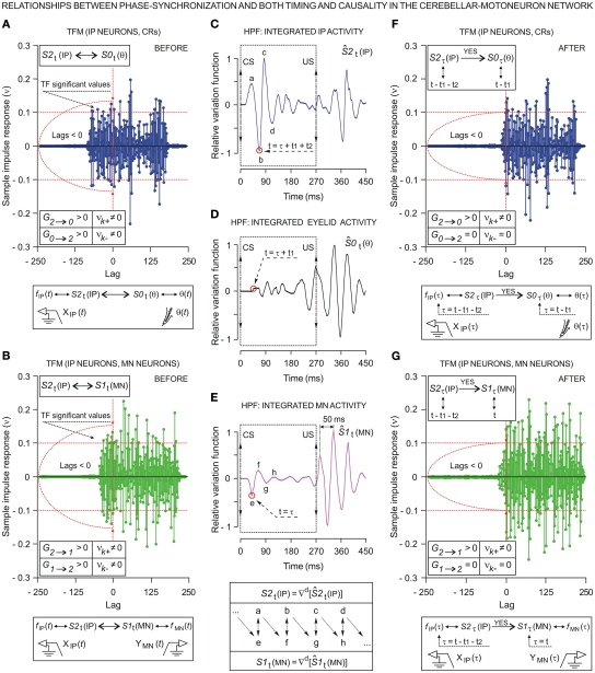
Figure 8.

Relationships between phase synchronization and both timing and causality in the cerebellar–Mn network using transfer function models (TFM) between kinetic neuronal commands of the IP neurons (IPn) and motor activities [activity of OO Mns (Mn) and eyelid CRs], before [see (A,B)] and after [see (F,G)] the phase synchronization as a simulated causal condition [see (C–E)]. (A,B) Before the phase synchronization, the transfer function models assume that the stationary time series S1_t (MN), S2_t (IP) and S0_t (θ) have a functional and dynamic relationship. In (A), the causality indices are such that G_2 → 0 > 0 and G_0 → 2 > 0, ν_k+ ≠ 0 and ν_k− ≠ 0 – i.e., S0_t(θ) depends on its own past and on the past of S2_t(IP), and S2_t(IP) depends on its own past and on the past of S0_t(θ). In (B), S1_t(MN) depends on its own past and on the past of S2_t(IP), and S2_t(IP) depends on its own past and on the past of S1_t(MN) – i.e., significant values of the causality indices in both senses: G_2 → 1 > 0, G_1 → 2 > 0, ν_k+ ≠ 0 and ν_k− ≠ 0. The transfer function models in (A,B) indicate the feedback relationships between IPn time series S2_t (IP) and either S0_t (θ) or S1_t (MN), at least in the statistical sense of causality. (C–E) Oscillatory curves (relative variation functions) resulting from high-pass filtering (HPF, –3 dB cutoff at 5 Hz and zero gain at 15 Hz) of integrated neuronal firing activities (IPn and Mn) and of eyelid position corresponding to the same set of records. The operator £^d enabled the stationary time series S1_t (MN), S2_t (IP), and S0_t (θ) to be obtained after making n = d regular differentiations to the non-stationary time series [i.e., the relative variation curves, as shown in (C–E)]. Note that in the oscillating curves shown here, components a–d are totally out-of-phase with components e–h. The transfer function models (F,G) assume that the stationary time series possess a direct interdependence after phase synchronization as a simulated causal condition [i.e., the phases corresponding to τ = t − t1 − t2, for S2_τ (IP), τ = t − t1, for S0_τ (θ), and τ = t, for S1_τ (MN)], implying that S0_τ (θ) depends on its own past and on the past of S2_τ (IP) (i.e., the indices are such that G_2 → 0 > 0 and G_0 → 2 = 0, ν_k+ ≠ 0 and ν_k− = 0, see F for a unidirectional coupling); and that S1_τ (MN) depends on its own past and on the past of S2_τ (IP) (i.e., G_2 → 1 > 0, G_1 → 2 = 0, ν_k+ ≠ 0, and ν_k− = 0, see the panel G for another unidirectional coupling). Red horizontal dashed lines in (A,B) and (F,G) indicate the approximate upper and lower confidence bounds (approximately 95% confidence interval), assuming the input and output physiological time series are completely uncorrelated.