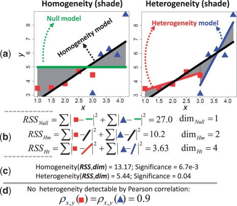
Fig. 1.

Computing heterogeneity and homogeneity of interactions across two conditions. Here, we use a linear interaction as an example. (a) In each condition, five independent noisy observations of random variables X and Y are provided. Condition 1 (red squares): (1.0,3.49), (1.5,3.53), (2.0,3.80), (2.5,4.68), (3.0,4.43); Condition 2 (blue triangles): (3.0,3.11), (3.3,5.89), (3.6,6.27), (3.9,5.85), (4.2,8.74). A null model is first obtained: y=4.98 (the green line). By pooling all 10 points, a homogeneity model (Hm) is obtain: y=0.9x + 2.27 (the black line). Then we obtain the heterogeneity model (Ht) which contains y=0.61x + 2.77 (the red line) and y=3.74x − 7.49 (the blue line), estimated from each group of 5 points, respectively. (b) The three models are evaluated by residual sum of squares (RSS) and model complexities via parameter dimensions (dim). (c) Finally, we compute the homogeneity and heterogeneity of the interaction between X and Y across conditions. They are related to the shaded area in the left and right panel in (a). The significant homogeneity indicates a common interaction trend; the significant heterogeneity suggests a difference between the two lines in the heterogeneity model, evidenced by a difference in slope. (d) In contrast, the difference in slope between the two models is undetectable by differential correlation, as difference between the Pearson's correlation coefficients across the two conditions is zero.